An Accelerated Cue Combination Principle Accounts for Multi-cue Depth Perception

Christopher W. Tyler

doi:10.2352/J.Percept.Imaging.2020.3.1.010501

Abstract

For the visual world in which we operate, the core issue is to conceptualize how its three-dimensional structure is encoded through the neural computation of multiple depth cues and their integration to a unitary depth structure. One approach to this issue is the full Bayesian model of scene understanding, but this is shown to require selection from the implausibly large number of possible scenes. An alternative approach is to propagate the implied depth structure solution for the scene through the “belief propagation” algorithm on general probability distributions. However, a more efficient model of local slant propagation is developed as an alternative.

The overall depth percept must be derived from the combination of all available depth cues, but a simple linear summation rule across, say, a dozen different depth cues, would massively overestimate the perceived depth in the scene in cases where each cue alone provides a close-to-veridical depth estimate. On the other hand, a Bayesian averaging or “modified weak fusion” model for depth cue combination does not provide for the observed enhancement of perceived depth from weak depth cues. Thus, the current models do not account for the empirical properties of perceived depth from multiple depth cues.

The present analysis shows that these problems can be addressed by an asymptotic, or hyperbolic Minkowski, approach to cue combination. With appropriate parameters, this first-order rule gives strong summation for a few depth cues, but the effect of an increasing number of cues beyond that remains too weak to account for the available degree of perceived depth magnitude. Finally, an accelerated asymptotic rule is proposed to match the empirical strength of perceived depth as measured, with appropriate behavior for any number of depth cues.

jpi

Journal of Perceptual Imaging

J. Percept. Imaging

2575-8144

Society for Imaging Science and Technology

jpi0118

10.2352/J.Percept.Imaging.2020.3.1.010501

0118

Regular Articles

An Accelerated Cue Combination Principle Accounts for Multi-cue Depth Perception

Accelerated cue combination for multi-cue depth perception

TylerChristopher W.

Smith-Kettlewell Eye Research Institute and Division of Optometry and Vision Science, City University of London (UK)

cwtyler2020@gmail.com

Tyler

012020

010501-1

010501-9

2022019

2212020

2020

Abstract

ccc

2575-8144/2020/3(1)/010501/9/$00.00

printed

Printed in the USA

Introduction

The world in which we have to operate is three-dimensional (3D; or four-dimensional, if we include time variations), so it is critical that we have a thorough representation of its full-dimensional layout in order to be able to navigate it effectively. The manner in which two-dimensional (2D) depth cues are combined to provide a full-dimensional depth map of the world in which we operate has a deep history but no current resolution, to my knowledge. To illustrate the issue, consider the case of depth from texture in perspective projection (Figure 1). Li & Zaidi [1] show that radically different forms and degrees of depth structure are perceived as a function of the orientation of textural information relative to the depth structure being depicted. (Note that these plaids are derived from uniform sinusoidal gratings, so there is no noise to render a given orientation noisy of variable other than quantal fluctuations; hence an ideal observer should extract the same depth structure from each variant.) The one-dimensional perceived depth profile for one observer (the author) is depicted in the green traces above each texture. (Li & Zaidi used an ordinal measure of depth structure, so their data cannot be used for quantitative comparisons of the strength of the depth percept.) The full texture is an 8-orientation (8-O) plaid depicting a three-cycle sinusoidal depth structure in perspective. The subsequent textures are a reduced plaid of just the vertical (V) and the (modulated) horizontal (H) orientations alone, the combined horizontal and vertical (H + V) plaid, and the full 8-O plaid. Physically, each separate orientation contains the full information about the geometric depth structure, but it can be seen that the depth effect is much stronger for the H than for the V orientation and that the effect is roughly additive for the two combined into an H/V plaid. Including the other six orientations for the 8-O plaid, however, does not further enhance the perceived depth, but tends to slightly reduce it. (The oblique components alone also elicited strong depth structure percepts [1]).

Figure 1.

Examples of static textures of different orientation compositions, all depicting the same physical three-cycle depth structure modified from Li & Zaidi [1], but giving very different strengths of perceived depth from texture as indicated in the profiles above each texture (with the upward direction coding “far depth”). The three-cycle geometric depth structure used to compute the texture perspective modulations is shown at far left. Weak depth is evoked by the vertical-stripe texture (especially if viewed close to avoid the spurious shading cue). Strong depth is seen for the (perspectively modulated) horizontal-stripe texture. Strong depth is seen for both the 2- and 8-orientation plaids.

The point of the demo in Figure 1 is to illustrate the concept of depth cue combination and its rules of operation, not to focus on this specific example for quantitative analysis. Qualitatively, it shows that perceived depth is not controlled by an averaging process, for then the depth of (H + V) would be less than for H alone, whereas it is closer to an additive summation process. Conversely, the perceived depth cannot be controlled purely by a simple additive process because the perceived depth for the 8-O plaid should be (roughly) four times greater than for the 2-orientation (H + V) plaid, whereas here it operates close to an averaging principle. The contribution of the present work is to show that current theoretical treatments of depth cue combination are incapable of accounting for empirical depth cue combination results and to provide a general cue combination principle that can do so. This demo thus encapsulates the thorny issue of the cue combination principles of operation, as developed below.

Depth Cue Combination Theories: A Critique

The two main competing theories are undifferentiated Bayesian selection or the strong fusion model (Bülthoff & Yuille [2]; Nakayama & Shimojo [3]; Likova & Tyler [4]) and depth cue combination or weak fusion models (Landy et al. [5]; Maloney & Landy [6]). The strong fusion model is effectively a formalized version of the Gregorian theory of perceptual hypothesis testing (Gregory [7, 8]) that perception consists of the probabilistic match of prior perceptual hypotheses to the available data. Thus, the strong fusion model implies that we have a full 3(+)D representation of any scene (or scene component) that we might encounter in the world, and the task of perception is to select among the probabilistic matches of this array of 3+D models to any scene we may encounter. The “+” sign is included because many scenes may include motion, three dimensions of defining color encoding, texture encoding, and so on. (For example, color would be a defining perceptual attribute of the ripeness of fruit, or a national flag, and so on.)

2.1

Simple Linear Summation

The modified weak fusion (MWF) model [5, 6] is presented as operating with linear summation of the depth cues (as developed in more detail below), although it actually includes a normalization term (see Eq. 3) that makes it an averaging model that would provide no summation of multiple weak cues. Thus, it is important to understand that simple linear summation (red curve in Figure 2), which would allow for increasing perceived depth, D, as more cues are included, would radically overshoot the veridical level after more than a few cues, once there were enough cues to sum to the veridical level. On the other hand, the expected value of the MWF averaging model would never deviate from veridical perceived depth (green dashed curve in Figure 2), violating the results of many depth cue combination studies. Specifically, for the MWF averaging model with four equally weighted cues, (1 + 1 + 1 + 1)∕4 = 1, whereas for a linear summation model, 1 + 1 + 1 + 1 = 4. The prescription suggested to avoid this problem is to include some cues to flatness (di = 0), here exemplified as contributing with equal strength to any one depth cue (blue curve in Figure 2). Specifically, for the MWF averaging model with two equally weighted cues, (0 + 1)∕2 = 0.5, whereas for the true additive model 0 + 1 = 1, and the (equally weighted) depth would never be less than veridical. While including the flatness cue(s) does provide for some degree of depth enhancement through depth cue combination, the blue curve in Figure 2 shows that the enhancement is far too slow to reach the asymptotic veridical value even with as many as a dozen depth cues.

Figure 2.

Modeling perceived depth as a function of number of depth cues. Simple linear summation (red line) for set of equal weak depth cues (di = 0.2 in this example) takes five cues to reach the veridical level (D = 1) but then overshoots if further cues are added. MWF weighted summation (green dashed curve) assumes that all cues are veridical, so perceived depth should always remain veridical regardless of the number of depth cues. Adding a unitary flatness cue (d1 = 0; blue curve) to the MWF model produces a nonlinear asymptotic function that asymptotes slowly toward veridicality, but fails to reach it even with 12 depth cues.

Moreover, this option of incorporating cues to flatness only applies to the presentation of stimuli on (flat) visual displays. It does not apply to the perceived flattening of the known 3D environment in reduced cue situations, such as when closing one eye, because the 3D world has no cues to flatness. The MWF hypothesis of Landy et al. [5] is based on the assumption that each depth cue alone is in fact veridical, though noisy, and thus any combination of depth cues should give an unbiased (i.e., full depth) impression, though weighted to the least noisy cue. The fact that perceived depth is itself less than veridical at larger viewing distances in full-cue situations (Erkelens [9]), and that closing one eye reduces perceived depth in otherwise full-cue situations (in which there are no cues or priors to flatness!) invalidates the MWF model as presented. (Note that, in practice, when trying the one-eye-closure experiment, it is important to wait for, say, 10 s, to allow the memory of the binocular depth structure to dissipate before assessing the depth. The eye should then be re-opened to allow a direct comparison of the monocular view with the refreshed binocular view.)

2.2

Full Bayesian Cue Combination

The Bayesian concept is that the 3D map is derived by comparing the 2D information in the image to the 2D projections of all possible 3D scenes that we might encounter. The full Bayesian cue combination rule is then that the depth map is selected according to the best, or maximuma posteriori (MAP), estimate from among all possible scenes, given the image data impinging on the eyes that incorporates an array of depth cue information. Note that in most cases this perceptual 3D map selection is achieved within a few hundred milliseconds. The absurdity of this proposal become evident as soon as we realize the trillions of possible scenes that the human may encounter, and indeed the proportion of them that could conceivably reside in memory relative to the number that may be encountered for the first time. To quantify this in orders of magnitude, we may consider that the surface of the earth has an area of ∼500 trillion square meters, so if each square meter constitutes a different station point, and the effective field of view is 1 steradian, the total number of different views would be ∼6 quadrillion. Obviously, these assumptions can be adjusted to suit different conceptualizations of distinct scenes, but this calculation gives a first approximation to the scale of the Bayesian proposition.

If we assume that the human encounters a new scene every second or so, the maximum number of scenes that an adult could have encountered in a lifetime would be only of an order of one billion, or a miniscule fraction of the sextillion possible scenes, so there is no conceivable memory that could have established the basis for selecting from the possible scenes that could actually be encountered by an earthbound traveler. Thus, while the Bayesian model could possibly operate to tell us which of our everyday scenes of familiar territory we are encountering, there is no possibility that it can explain our ability to comprehend the depth map of any novel scene on earth that we might encounter.

Guided Hypothesis Testing or Mid-Level Constructive Bayesian Cue Interpretation

Since the full Bayesian approach is combinatorially implausible, is there a version of this theory that could plausibly be neurally implementable? To do so, we need to take into account that depth cues can be both sparse and ambiguous (Tyler & Kontsevich [10]; Tyler [11]). Rather than simply surveying trillions of possible scenes to find a match, it is far more plausible that the visual system uses some reliable depth information as a local starting point and follows a mid-level constructive Bayesian strategy of assuming that the scene is made up of a variety of surfaces extending from this local starting point to other points of reliable depth information (see Likova & Tyler [4]).

While still incorporating prior information about the structure of the world, this “constructive Bayesianism” is a far different proposition as to how the prior information is used (e.g., Su, Cormack, & Bovik [12]). By restricting the Bayesian priors to a succession of local options, it reduces the MAP implementation to a manageable number of choices. Once the local surface slant is determined, the constructive Bayesian approach would resemble the “search for dense surfaces” operation proposed by Julesz for solving the depth map of random-dot stereograms (RDS). Once started, the process could rapidly sample the local slant regions around the edge of the initial region, seeded by the slant of the initial region, thus reducing the choices to be sampled by many orders of magnitude if the surface is continuous through each new sample. In this way, the flexible Bayesian prior that the solution is a two-parameter surface can be used to construct the most likely surface implied by the concatenation of available depth cues. It has, in fact, been implemented as a computational algorithm for the binocular disparity cue by Sun, Zheng, & Shum [13].

3.1

Mathematical Development

Local Bayesian priors are typically implemented as “belief propagation” through what is known (confusingly) as a “factor graph”, but what will be termed here a belief propagation net (BPN). A “belief” is a probability distribution of the current local solution of the problem in hand (which is the depth map of the visual scene). Thus, for a depth propagation algorithm such as those of Sun, Zheng, & Shum [13] for disparity, of Potetz & Lee [14] for shading, etc., the current result of each iteration of the BPN is the distribution of the likelihood of each possible depth (from, say, 10 cm to ∞) at each node in the BPN. Such beliefs propagate by Bayesian multiplication such that:

(1)

\begin{matrix} p_{i, j} (d) & = & \prod (d_{i, j}, p_{i - 1, j - 1} (d), p_{i + 1, j - 1} (d), p_{i - 1, j + 1} (d), \\ p_{i + 1, j + 1} (d)), \end{matrix}

where the first element of the product operator Π is the initial input solution to the depth d at node i,j and the other four elements are the distributions of neighboring depth solutions on d.

If we replace the 2D index i,j with the more general index i of the successive neighbors around each node j (which generalizes to index any form of connectivity through the BPN), we have the general expression:

(2)

p_{j} (d) = \prod_{i = 1}^{k} (d_{j}, p_{i, j} (d)) .

This approach, however, is very computationally expensive and neurally implausible (e.g., [14]). A rather more efficient approach is to constrain the propagation of full distributions under the assumption that they approximate Gaussian distributions that can be characterized by their first two moments, the mean m and the reliability represented by the variance σ2. Thus, since the mean of the product of Gaussian is equal to the sum of their means weighted in inverse proportion to their σs, Eq. (2) becomes:

(3)

d_{j} (m, σ) = \frac{1}{k} (\sum_{i = 1}^{k} (m_{i, j} ∕ {σ^{2}}_{i, j}), [\sum_{i = 1}^{k} (σ_{i, j}^{2})]) .

The current proposal for guided hypothesis testing is, instead of propagating depth solutions, d, to propagate local slant solutions, s(θ, ϕ), such that:

(4)

\begin{matrix} s_{j} (m (θ, ϕ), σ (θ, ϕ)) = \frac{1}{k} (\sum_{i = 1}^{k} (\frac{m_{i, j} (θ, ϕ)}{{σ^{2}}_{i, j} (θ, ϕ)}), \\ [\sum_{i = 1}^{k} (σ_{i, j}^{2} (θ, ϕ))]), \end{matrix}

where sj(θ, ϕ) = dj(θ, ϕ) m − dj′(θ, ϕ) m, with j(θ, ϕ) being a net node adjacent to node j in direction (θ, ϕ) and i being the local slants at points adjacent to point j, excluding those in the direction of propagation [32].

3.2

Applications of the Constructive Bayesian Approach to Cue Combination

In particular, this constructive Bayesian approach can be used to extrapolate the surface over regions of indeterminate depth in sparse cue situations containing null, or NaN, values in the cue map. Where the null surface region is adjacent to local depth cue information, the Bayesian surface prior can be applied to the null, or NaN, regions in the form of the assumption that, in the absence of surface cues, the surface continues in the same orientation and depth as in adjacent regions where it was defined. This is the spatial equivalent of Newton’s first law of motion that objects will continue in straight-line motion unless perturbed by an external force. Here, the rule is that, unless perturbed by further depth cues, surfaces will continue to extend at a uniform slant throughout the scene (as looking at a large ground plane or wall), so the local slant is predictive of the extension over large regions, allowing for rapid propagation of local solution to large regions of the visual field. The property of surface continuity, and its extension to higher derivatives, allows for the extended use of mid-level Bayesian constraints in solving the depth construct problem [10].

The issue is complicated by the existence of transparent, translucent, and reflective surfaces, which incorporate multiple surface information along any visual direction line involved, such as in a wireframe cube or the ambiguous random-dot stereograms of Julesz & Miller [15]. The visual system now has to understand the multiple 3D surface structure of the scene in depth. Tyler & Kontsevich [10] argued that this structure is resolved serially through the construct of the attentional shroud, which first extrapolates to one surface structure (usually the nearest) and then the other, or others, one surface at a time. The same process is proposed for monocular depth cues to multiple surface structure such as the Necker cube, which is seen first protruding in depth and then receding, in alternating flips. The percept of the cube is inherently a three-dimensional one, but it is notable that the solutions are only seen one at a time.

In summary, this conceptualization may be expressed as Tyler’s Rules of Visual Surface Structure:

Changes in physical surface slant tend to be accompanied by changes in depth cue information.

In the absence of perturbing depth cues, the slant of a surface region is equal to the slants of its adjacent regions.

Transparent and reflective surfaces may incorporate multiple surface information along any visual direction line.

Beyond Weak Fusion Cue Combination

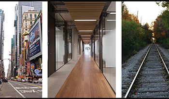
In terms of slant, the standard starting point is the MWF theory of cue combination of Landy, Maloney, and colleagues [5, 6, 16–18], which is considered to be the reigning theory of depth cue fusion. As confirmed with them, MWF is not a meaningful theory for depth as experienced in the world, because perceived depth deviates radically from the veridical estimate. This can be seen in any view down a parallel street, corridor or railroad track (Figure 3), in each of which the perspective is seen as converging rather than parallel, indicating that the depth impression is reduced relative to its veridical extent. (This converging perspective impression is expected in the printed illustrations, which have both binocular and textural cues to flatness, but viewing similar scenes in the full-cue context of everyday life will verify that they are still seen with converging perspective.)

Figure 3.

Perspective views of Times Square, an office corridor and a railroad track. Each evokes a substantial depth impression when fixating the vanishing point, but a pronounced degree of perceived convergence remains. Even in the full-cue situation of real-life viewing of such scenes, the perspective is still seen as converging rather than parallel, indicating that the full-cue depth impression is reduced relative to its veridical extent.

The lines always appear to converge to some extent, even though we know that they must be parallel and treat them as such motorically as we navigate through these environments. Although we may be able to estimate the metric distance by cognitive training, the visual structure of the everyday full-cue scene always appears to be at least somewhat trapezoidal toward the vanishing point rather than the fully parallel rectanguloid shape of its physical structure. This distorted visual impression establishes that the perceived depth is never veridical in such full-cue distance perception, as has been determined empirically by Erkelens [9], who provides a perspective-space model for these effects that is able to simultaneously predict the perceived, distances, sizes, and angles of full-cue scenes by means of the single parameter of the distance of the vanishing point.

4.1

Mathematical Development

This result is significant because the prevailing weak fusion theory is that the overall perceived depth D is a Gaussian-reliability weighted linear sum of the veridical depths from individual depth cues, c [5, 17]

(5)

D = \sum_{c} d_{c} ∕ σ_{c}^{2}, where \sum_{c} 1 ∕ σ_{c}^{2} = 1, and \sum_{c} d_{c} = 1 forall c,

and where the dc in their theory are assumed to be veridical readouts of the depths.

In other words, they assume that ∑ dc = 1 for all c, which means that D = 1 for all combinations of weights (meaning that all depth estimates are noisy but always veridical on average). So, as expressed in Landy, Maloney, & Young [5], the theory only predicts the variance of each depth cue, but does not allow for any form of reduced depth percept as is experienced in the world. This seems a severe limitation, since many depth cue measures show non-veridical depth perception from individual cues, including those in their own studies (such as Johnston et al. [19], see Figure 4).

Figure 4.

Illustration of the asymptotic and accelerated asymptotic depth cue combination rules, under the assumptions that they have equal Bayesian weights of 0.5 of the Bayesian norm for the depth of the depicted object.

More specifically, Landy, Maloney, & Young, [16] and Landy et al. [5] structure their MWF theory to apply locally to all points in the visual field:

(6)

\begin{matrix} D (x, y) = \sum_{c} \bar{d_{c}} (x, y) ∕ σ_{c}^{2} (x, y), \\ where \sum_{c} 1 ∕ σ_{c}^{2} (x, y) = 1, forall (x, y), \end{matrix}

and where the bar over the dc variable represents its mean over the parameter used to estimate the variance such as time samples (which is unspecified in the cited sources).

By doing so, the authors imply both that the reliability weighting differentially affects the mean perceived depth at each (x, y) location in the visual field, and that this local effect on the perceived depth contribution from any one depth cue, c, is affected by the reliability at that location in all other depth cues.

4.2

Implications of the Modified Weak Fusion Theory

This particularity of the MWF theory thus implies that the depth structure of the scene will vary locally across the scene, which seems to predict complex fluctuations in the perceived depth over time as the reliability for each local region is defined. They do not specify the time constant of the reliability estimation (or even whether it has a time constant), but in order to be applicable to real-life viewing of visual scenes, the reliability estimation would have to have a time constant as short as 300 ms, the average time between saccades to different points in a visual scene. If it were any longer, the reliability estimation would persist across saccades to inappropriate regions of the current visual space, where a different scene structure had prevailed prior to the saccade. For these reasons, it seems much more plausible to assume that the reliability is estimated across the scene as a unitary variable for each depth cue, c (Eq. (5)).

Conversely, there are situations in which depth perception is known to vary locally, principally when viewing unfamiliar random-dot stereograms (RDS; Julesz [20]). In such cases, the depth may be perceived as appearing in one region while it initially remains incoherent in other regions. The depth surface then appears to spread out from the seeded core, either with or without the aid of eye movements (Saye & Frisby [21]). This could be regarded as some form of MWF integration as the continued sampling of the local image builds up the reliability of the local depth estimates. However, it is not clear that this is a valid interpretation because the visual image is not changing as viewing time increases (in the case of static RDS). The same array of “valid” and “spurious” (or intended and unintended) local disparities activates the array of local disparity detectors at each point in the RDS image over time. What is happening neurally is that the depth surface solution in one region seeds the solution in an adjacent region (Samonds, Tyler, & Lee [22]) in a form of “belief propagation” or local Bayesian prior refinement rather than a reduction in the reliability of the local signals, per se. Thus, the MWF relationship of Eq. (6) should be restructured to reflect the sequential propagation of the local prior from regions where a solution has been found to adjacent regions. It is interesting that this perceptual behavior tends to asymptote with repeated viewing to an ability to see the whole stereoscopically depicted surface rapidly in a single glance (Goryo & Kikuchi [23]; MacCracken, Bourne, & Hayes [24]), implying that the depth surface prior becomes an accessible memory trace that can be activated immediately on re-viewing the particular RDS, even many weeks or months later.

Landy, Maloney, & Young [16] do not specify what happens for situations like pictorial depth or “reverspectives” (physical images that counteract real slants with reversed perspective patterns), but here the theory would not apply because the depth cues are discrepant, with some being zero or negative, and hence do not conform to their restriction that the theory only applies where the differential cues are not too discrepant. This is why Young, Landy, & Maloney [17] implemented a Perturbation Theory of depth cue combination, because they allow small perturbations around the veridical depth values to test their theory, but not large discrepancies.

However, this restriction essentially implies that their formulation of the MWF cue combination theory Eq. (6) does not apply to real-world depth perception in general, because the perceived depth in the world derives from the full scope of twelve or more depth cues (Trommershauser, Kording, & Landy [25]: Goldstein & Brockmole, [26] p. 229) some of which are much weaker than others (e.g., Likova & Tyler [4]), particularly in situations where there is only sparse information for a particular cue. In Chen & Tyler [27], for example, we showed that disparity carried by typical luminance shading cues is about 4x weaker than the monocular shading cue in generating perceived depth, and as much as 30x weaker than full-spectrum disparity information depicting the same shading surface. Application of the theory to such situations, and also for all depth perceived in pictures, print or electronic displays is forbidden by this restriction, leaving us with no viable theory for many of the predominant cases for depth perception. On the other hand, under the weighted averaging principle of MWF, multiple unbiased depth cues per se do not add up, by definition, to more than veridical depth.

Where the theory can provide some degree of promotion is in situations where some depth cues are reliable cues to flatness, rather than veridical depth structure (Yuille & Bülthoff [28]; Saunders & Chen [29]). However, in the data from Johnston, Cumming, & Landy [19] that are serving as the testbed for the present analysis, disparity and motion cues are weakened in some cases by cue-specific manipulations that do not change the configuration of the competing cues to flatness, as would be required by MWF. And they do not provide a quantitative account of the promotion that they observe in the MWF framework. In both these respects, the MWF framework is incomplete. (In principle, depth cues can be scaled according to an appropriate function of their controlling variables such as vergence angle for disparity or head velocity for motion parallax, as discussed by the MWF proponents, but such functions are not implemented in their formal analyses. Such scaling would be termed “biasing” in their terminology, and is formally incompatible with their unbiased theoretical framework for cue combination.)

4.3

A Practical Depth Cue Combination Rule

In the context of these problems with the MWF model, a more realistic approach to depth cues might be to regard them as modulations around Gogel’s [30] specific distance tendency (SDT) of ∼1.5 m, which has various manifestations (including a specific distance of the internal screen with eyes closed).

(7)

D (x, y) = S D T + \sum_{i} [\bar{d_{i}} (x, y) ∕ (1 + {\bar{σ}}_{i}^{2} (x, y))] .

In this formulation, a cue is not fully veridically expressed unless its variance is zero, but veridicality is closely approximated when

{\bar{σ}}_{i} ≪ 1

The operating philosophy of the brain seems to be to treat single depth cues as unreliable but to place strong weight on converging evidence from multiple depth cues (Yuille & Bülthoff [28]). This approach suggests that the depth map can be constructed from some form of Bayesian combination of all possible depth maps from the multiple cues. The problem is that, in order to specify the depth structure of the visual scene, we need to decode the depth information from the variety of available depth cues, many of which are inherently sparse across space. All depth cues are sparse wherever the scene has uniform shading. Additionally, disparity and motion cues are sparse wherever a correspondence cannot be established. This is where the cues would need to be filled in by the mechanism of interpolation to generate the resultant depth map (Likova & Tyler [4]), perhaps with feedback down to the early areas again.

A key point is the depth scaling for each of the depth cues. Note that, if they are sparse, they are subject to discontinuities between the depths specified by each of the cues, unless they are all consistently scaled. Disparity cues are scaled by the convergence angle, which is a joint function of interocular distance and convergence distance. Motion parallax cues are scaled by the rate of head motion and the fixation distance. As Belhumeur et al. [31] showed, the shading cue is subject to a bas-relief ambiguity (although this may be resolved by the self-illumination cues). Texture cues are scaled by the absolute texture size. Thus, there is no unitary scaling variable for the various depth cues, and the cue combination map must have a rescaling mechanism by which to combine the sparse cues for minimum mismatch in the resultant depth map. It presumably relies on a set of default assumptions (Bayesian priors) that it brings to the typical situation, but has the ability to rescale the variables when encountering unusual situations.

Thus, a more realistic rule might be a hyperbolic asymptotic formulation:

(8)

D = [1 - 1 ∕ \frac{(\sum_{1}^{k} [d_{z} (x, y) ∕ (a_{z} \cdot {\bar{σ}}_{z}^{2})])}{\sum_{1}^{k} {\bar{d}}_{z}}]

where z = 1 : k indexes the depth cues.

This function has the effect of summing over the depth cues up to the veridical depth that determines the asymptotic summation value of multiple cues. The cue-specific scaling constant az represents the degree to which each depth cue is a non-veridical Bayesian norm even in the absence of competing cues. Note that this is a model of the perceived depth in the absence of cognitive priors, not of the fully cognitive distance estimation. (For example, when you look at the images of Figure 3 monocularly, they may evoke a sense of several inches of depth into the page (or screen), with a reduced effect when viewing binocularly. Cognitively, you know that there is actually zero depth, but you also know that it is a picture of a parallel-sided corridor with a depth of many meters. Thus, although you have a single—though possibly time-varying—depth percept, it evokes an interplay among multiple cognitive interpretations of what the depth structure “actually” is depicted.)

The resultant framework can account for a general weakness in individual depth cues, since the weighted average will always fall somewhere between the extreme values being combined. However, if all depth cues are individually weak, it cannot account for the tendency of depth cues to reinforce each other to provide a veridical representation. This reinforcement is captured by a hyperbolic Minkowski rule for the cue combination:

(9)

\begin{matrix} D & = & 1 - 1 ∕ [{(\sum_{1}^{k} \frac{σ_{z}^{2}}{k})}^{\frac{p}{2}} . ({(\sum_{1}^{k} \frac{d_{z} ∕ a_{z}}{k . σ_{z}^{2}})}^{\frac{p}{2}} \\ + {(\sum_{1}^{k} \frac{d_{0}}{k . σ_{z}^{2}})}^{\frac{p}{2}})], \end{matrix}

where d0 is the SDT for each depth cue that includes priors from set points on vergence and accommodation cues, and the Minkowski exponent p is a free parameter of the model.

The simple asymptotic (blue dashed line) and accelerated asymptotic (full red line) principles for multiple depth cue combination are illustrated in Figure 4 for the particular case that the net Bayesian weights are equal for all depth cues and the Minkowski exponent is an empirical parameter set to p = 6 for the present case. (The equations apply for all varieties of the combinations of inherent cue values and their associated Bayesian weights, but the case of equal net weights is the most straightforward form to illustrate.) The simple asymptotic principle (blue dashed curve) achieves the result that individual weak depth cues do not add up to supranormal depth representation when many cues are combined (as they would for simple linear summation as soon as the number of cues exceeded their strength relative to the veridical level), nor do they average to the same net value as the individual cues (as they would for a literal averaging principle). Instead, the simple asymptotic values increase toward the Bayesian norm value that presumably approximates the veridical depth value, if past experience is an accurate guide.

However, as illustrated by the blue dashed curve in Figure 4, the simple hyperbolic function of Eq. (8) does not satisfactorily reach asymptote for even a large number of consistent depth cues, whereas the experimental results discussed in the following require an accelerated cue combination rule such as that of Eq. (9), illustrated for the specified parameters by the red curve in Figure 4. This equation now provides for the requisite rapid achievement of the Bayesian norm level with two or three consistent depth cues, while avoiding both supernormal summation or the failure to reach asymptote for many cues.

Quantitative Comparison of Cue Combination Principles

These two asymptotic principles can be compared with the data of Johnston, Cumming, & Landy [19] for depth estimation of elliptical cylindrical figures defined by disparity and motion cues, by setting them to appear as the criterion shape of circular cylinders. These data were not in fact modeled in any of the co-authors’ publications even though they provide a strong test of their theoretical framework. Their data for three participants, transformed as the reciprocals of the adjusted depth matches to provide estimates of the strength of depth percepts, are shown in Figure 5. The cue combination results (red bars) are compared with the predictions of the Bayesian averaging rule of Eq. (5) (orange bars and horizontal red lines) and the present accelerated asymptotic principle of Eq. (9) (pink bars) for full-cue conditions (leftmost panel), and also with the combinations of two conditions to weaken the stereo cue (the 200 cm viewing distance), the motion cue (only two-frame motion), or both. The key target is the prediction of the perceived depth in the combined stereo and motion condition (red bars) from those in the separate stereo only, and motion only, conditions (blue and green bars, respectively). It can be seen that the Bayesian averaging fails to capture the tendency for enhanced depth from the combined cues (as recognized by the authors of the study), whereas the Accelerated Asymptotic prediction is accurate within experimental error because it provides for the significant promotion of the perceived depth from the combinations of weak depth cues.

Figure 5.

The stereo + motion depth matching data of Johnston, Cumming, & Landy [19], replotted as adjusted depth matches, compared with their Bayesian averaging rule (orange dashed bars and red lines) and the accelerated asymptotic principle of Eq. (9) (pink dashed bars). Blue bars—depth from stereo only; green bars—depth from motion only; red bars—depth from stereo + motion (S + M). Note that the Bayesian averaging rule produces poor predictions when both depth cues are weakened, whereas the accelerated asymptotic principle matches the data in all conditions within experimental error.

The most important case is that of the fourth panel of Figure 5, showing veridical depth perception for the combination of two cues weakened to the 50% level, which implies that only a process providing for linear summation from just these two cues (without the reweighting constraint that the weights should sum to 1) can account for this behavior, implying that no third cue to flatness was involved. More specifically, from Eq. (5), we have:

(10)

D_{1} = d_{1} ∕ σ_{1}^{2} + ε, D_{2} = d_{2} ∕ σ_{2}^{2} + ε,

where d1 and d2 are the two individual depth cues, and ε is the contribution of any residual cues to flatness (which were minimized as far as possible in this experimental situation). Since the data show that D1 = D2 = ∼ 0.5 for both conditions, it implies that:

(11)

(d_{1} ∕ σ_{1}^{2} + ε) + (d_{2} ∕ σ_{2}^{2} + ε) = 1

and that:

(12)

D_{1 + 2} = d_{1} ∕ σ_{1}^{2} + d_{2} ∕ σ_{2}^{2} + ε = 1 .

Hence:

(13)

d_{1} ∕ σ_{1}^{2} + ε + d_{2} ∕ σ_{2}^{2} + ε = d_{1} ∕ σ_{1}^{2} + d_{2} ∕ σ_{2}^{2} + ε

and thus:

(14)

2 ε = ε

which is only true if:

(15)

ε = 0 .

Thus, under the assumptions of an unconstrained linear model, the quantitative values of the fourth panel of Figure 5 are compatible only with the conclusion that cues to flatness played no role in the perceived depth, which is therefore inconsistent with the MWF model.

Conclusion

The analysis shows that, although the net depth percept must be derived from the combination of information from all available depth cues, a simple linear combination rule will drastically overestimate the perceived depth in the scene in cases where each cue alone provides a close-to-veridical depth estimate. On the other hand, the predominant model of Bayesian averaging, or the “modified weak fusion” model of depth cue combination, does not provide for the observed enhancement of perceived depth magnitude from weak depth cues. These problems can be addressed with an Accelerated Asymptotic rule that shows strong summation for two or three depth cues but rapidly asymptotes toward the full-cue level beyond that number of depth cues. This model is validated on published cue combination data that are inconsistent with the predictions of the “modified weak fusion” model. This analysis therefore lays the groundwork for more realistic assessment of human depth perception characteristics in both the full-cue situation of the everyday world and the reduced and/or conflicting depth cue situation of the ubiquitous visual displays of the artificial environment.

Acknowledgment

The author thanks Larry Maloney and Mike Landy for discussions on the implications of the MWF model of depth cue combination. This work is supported by AFOSR FA9550-09-1-0678 to CWT and NSF 1640914 to LT Likova.

References

1LiA.ZaidiQ.2000Perception of three-dimensional shape from texture is based on patterns of oriented energyVis. Res.40217242217–4210.1016/S0042-6989(99)00169-8

2BülthoffH. H.YuilleA. L.SchenkerP. S.1991Shape-from-X: Psychophysics and computationSensor Fusion III: 3D Perception and Recognition235246235–46International Society for Optics and Photonics

3NakayamaK.ShimojoS.1992Experiencing and perceiving visual surfacesScience257135713631357–6310.1126/science.1529336

4LikovaL. T.TylerC. W.2003Peak localization of sparsely sampled luminance patterns is based on interpolated 3D object representationsVis. Res.43264926572649–5710.1016/S0042-6989(02)00575-8

5LandyM. S.MaloneyL. T.JohnstonE. B.YoungM.1995Measurement and modeling of depth cue combination: In defense of weak fusionVis. Res.35389412389–41210.1016/0042-6989(94)00176-M

6MaloneyL. T.LandyM. S.1989A statistical framework for robust fusion of depth informationSPIE Proc.1199115411641154–64

7GregoryR. L.1963Distortion of visual space as inappropriate constancy scalingNature199678680678–8010.1038/199678a0

8GregoryR. L.1980Perceptions as hypothesesPhil. Trans. Royal Soc. Lond. Biological Sciences B290181197181–9710.1098/rstb.1980.0090

9ErkelensC. J.2015The extent of visual space inferred from perspective anglesi-Perception65145–1410.1068/i0673

10TylerC. W.KontsevichL. L.1995Mechanisms of stereoscopic processing: stereoattention and surface perception in depth reconstructionPerception24127153127–5310.1068/p240127

11TylerC. W.2004Theory of texture discrimination based on higher-order perturbation in individual texture samplesVis. Res.44217921862179–8610.1016/j.visres.2004.03.029

12SuC. C.CormackL. K.BovikA. C.“Bayesian depth estimation from monocular natural images,” J. Vis. 17, 1–29 (2017)

13SunJ.ZhengN. N.ShumH.-Y.2003Stereo matching using belief propagationIEEE Trans. Pattern Anal. Mach. Intell.25787800787–80010.1109/TPAMI.2003.1206509

14PotetzB.LeeT. S.2003Statistical correlations between 2D Images and 3D structures in natural scenesJ. Opt. Soc. Am. A20129213031292–30310.1364/JOSAA.20.001292

15JuleszB.MillerJ. E.1991Automatic stereoscopic presentation of functions of two variablesBell Syst. Tech. J.41663676663–7610.1002/j.1538-7305.1962.tb02424.x

16LandyM. S.MaloneyL. T.YoungM. J.SchenkerP. S.Psychophysical estimation of the human depth combination ruleSensor Fusion III: 3D Perception and Recognition1991International Society for Optics and Photonics247255247–55

17YoungM. J.LandyM. S.MaloneyL. T.18A perturbation analysis of depth perception from combinations of texture and motion cuesVis. Res.33268526962685–9610.1016/0042-6989(93)90228-O

18OruçI.MaloneyL. T.LandyM. S.2003Weighted linear cue combination with possibly correlated errorVis. Res.43245124682451–6810.1016/S0042-6989(03)00435-8

19JohnstonE. B.CummingB. G.LandyM. S.1994Integration of stereopsis and motion shape cuesVis. Res.34225922752259–7510.1016/0042-6989(94)90106-6

20JuleszB.Foundations of Cyclopean Perception1971U. Chicago PressOxford, England

21SayeA.FrisbyJ. P.1975The role of monocularly conspicuous features in facilitating stereopsis from random-dot stereogramsPerception4159171159–7110.1068/p040159

22SamondsJ. M.TylerC. W.LeeT. S.“Evidence of stereoscopic surface disambiguation in the responses of V1 neurons,” Cereb. Cortex 27, 2260–2275 (2017)

23GoryoK.KikuchiT.1971Disparity and training in stereopsisJapan. Psychological Res.13148152148–5210.4992/psycholres1954.13.148

24MacCrackenP. J.BourneJ. A.HayesW. N.1977Experience and latency to achieve stereopsis: A replicationPerceptual and Motor Skills45261262261–210.2466/pms.1977.45.1.261

25TrommershauserJ.KordingK.LandyM. S.Sensory Cue Integration2011Oxford University PressOxford

26GoldsteinE. B.BrockmoleJ.Sensation and Perception201610th ed.Cengage LearningBoston MA

27ChenC. C.TylerC. W.2015Shading beats binocular disparity in depth from luminance gradients: Evidence against a maximum likelihood principle for cue combinationPLoS One10e013265810.1371/journal.pone.0132658

28YuilleA. L.BülthoffH. H.KnillD. C.RichardsW.1995Bayesian decision theory and psychophysicsBayesian Perspectives on Visual PerceptionCambridge University PressCambridge

29SaundersJ. A.ChenZ.“Perceptual biases and cue weighting in perception of 3D slant from texture and stereo information,” J. Vis. 15, 1–24 (2015)

30GogelW. C.1969“The sensing of retinal size,” Vis. Res. 33, 173–193 (1969)

31BelhumeurP. N.KriegmanD.YuilleA. L.1999The bas-relief ambiguityInt. J. Comput. Vis.35334433–4410.1023/A:1008154927611

32TylerC. W.GopiA.Computational estimation of scene structure through texture gradient cuesIS&T Electronic Imaging: Human Vision and Electronic Imaging2017IS&TSpringfield, VA167176167–76