(1) Real vehicle experiment (Experiment 1)

In regard to the three levels of motion sickness, there were 85 cases of 1 (No sickness), 31 cases of 2 (Slight Sickness), and 1 case of 3 (High Sickness). The transition of motion sickness for each time interval is shown in Figure 3 on Experiment 1. In the plots, the horizontal axis indicates the time interval, and the vertical axis indicates the average of motion sickness in all participants. Significant differences were seen in one-way repeated measures ANOVA with time interval (F(12,96) = 2.216, p = 0.017, and η2 = 0.109). Shaffer post-hoc paired test with time factor was conducted but there were no significant differences.

(2) Stereoscopic visual simulation

In regard to the three levels of motion sickness, there were 456 cases of 1 (No sickness), 196 cases of 2 (Slight Sickness), and 24 cases of 3 (High Sickness). The transition for each time interval is shown in Fig. 3 on Experiment 2. In the plots, the horizontal axis indicates the time interval, and the vertical axis indicates the average of motion sickness in all participants. Significant differences were seen in one-way repeated measures ANOVA with time interval (F(12, 612) = 11.736, p < 0.001, and η2 = 0.090). Shaffer post-hoc paired test with time factor showed significant differences in Time 0-10 sec (T1)–T9, T10, T13, T2–T7, T8, T9, T10, T11, T12, T13, T3–T7, T8, T9, T10, T13, T4–T9, T10, T13, T5–T10, T13, T6–T10, and T13 (Table A1 and Table A2).

To judge the correspondence with the subjective indicators, we calculated the mean value of each indicator, using 10 s as an interval. Additionally, the objective indicators used were EDA, pulse rate, and LF/HF, and each participant was normalized from −1 by MinMaxScaler to see the variation.

For the model to predict motion sickness, a deep learning model based on one-dimensional convolutional neural network (1DCNN) was used. The prediction was performed using a recurrent neural network (RNN); however, as the 1DCNN model had higher precision, we reported the 1DCNN model results. The model had three layers–convolution, pooling, and dropout–and two fully connected layers. In the first fully connected layer, we input the predicted value for motion sickness in the previous interval. Leaky ReLU was used as the activation function, and Softmax was used as the output layer. The categorical cross-entropy loss function and Adam optimization algorithm were used. An image of the model is shown in Figure 7.

Data with missing values were excluded, so datasets were for 9 people in Experiment 1 and 52 in Experiment 2 and the data were divided every 10 s to predict motion sickness levels. For objective indicators, EDA, pulse rate, and LF/HF were used. Each indicator was normalized in the MinMaxScaler as −1–1 for each participant. When predicting motion sickness, as there were few cases of 3 (High Sickness), it was considered to be 0 (No sickness) as 1 (No Sickness), and 1 (Sickness) as 2 (Slight Sickness) and 3 (High Sickness). So that the data of Experiment 1 is based on 85 cases of 0, 32 cases of 1, and the data of Experiment 2 is based on 456 cases of 0, 220 cases of 1.

For accuracy verification, the average value of the results in four-fold cross-validation randomly in person and time was used. A summary of the confusion matrix of the four sessions is shown in Table II. The mean accuracy of the four sessions was 0.833, with the F1-score for “Nothing” being 0.883 and F1-score for “Sickness” being 0.684.

For accuracy verification, the average value of the results in the four-fold cross-validation randomly in person and time was used. A summary of the confusion matrix of the four sessions is shown in Table III. The mean accuracy for the four sessions was 0.844, with the F1-score for “Nothing” being 0.885 and F1-score for “Sickness” being 0.745.

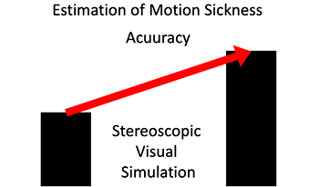
To validate the effect of expanding the training data from Experiment 2, a four-fold cross-validation was performed on Experiment 1 data. The data from the stereoscopic video experiment was also added to the training data (Figure 8). A summary of the confusion matrix for the four sessions is shown in Table IV. The mean accuracy for the four sessions was 0.866, with the F1-score for “Nothing” being 0.896 and F1-score for “Sickness” being 0.754.

It is known that the user experience changes with viewing time in VR [22]. Thus, the effect of time and somatosensory information was analyzed by comparing Experiment 1 and Experiment 2. The results of the actual vehicle experiment demonstrated a tendency for motion sickness to increase, with a peak at the 110-s interval. The results of the stereoscopic visual experiment demonstrated a tendency for motion sickness to increase, with a peak at the 100- and 130-s intervals. Where each experiment demonstrated an increasing trend, the fact that the position of the peak differs is thought to be due to the fact that the degree of sensory conflict differs in the various cases of vehicle sickness and simulation sickness. Particularly, it is affected by the presence or absence of somatosensory information being presented.

Compared to the real vehicle experiment, each indicator in the stereoscopic visual experiment tended to vary by only a small degree. In the results of ANOVA for the real vehicle experiment, a large effect size was seen for EDA and HR, whereas a small effect size was seen for LF/HF bands. Furthermore, in the results of ANOVA for the stereoscopic visual experiment, a small degree of change was seen for all participants. This suggests that the response of the objective index was greater for the real vehicle than for the stereoscopic visuals.

If we compare the peak positions for the objective and subjective indicators, we can see that the peak position does not match for any participants. This suggests that evaluating the response to specific objective indicators and subjective indicators is difficult.

The cross-validation accuracy of the real vehicle test was 0.833, and the cross-validation accuracy of the stereoscopic visual experiment was 0.844. When the learning data used in the stereoscopic visual experiment was extended, the cross-validation accuracy was 0.866. In a previous study, predicting the motion sickness levels through a self-organizing neural fuzzy inference network (SONFIN) using EEG signals, an overall accuracy of about 82% through experiments was achieved [23]. When predicting motion sickness levels through a three-dimensional convolutional neural network (3DCNN) using 3D image information, the correlation between a simulator sickness questionnaire (SSQ) [24] and prediction score was 0.845 [25]. When predicting the VR sickness levels through a Deep Long Short Term Memory Model (LSTM) using posture instability signal, the correlation between a SSQ and prediction score was 0.89 [26]. These results suggest that the accuracy for predicting motion sickness within the respective tests could be predicted with constant accuracy. Therefore, it is thought that the objective indicators obtained in this study can contribute to predicting motion sickness to some extent. Additionally, by adding the stereoscopic visual simulation data to the real vehicle experiment, it was confirmed that the accuracy for predicting motion sickness in the real vehicle experiment could be improved. Thus, even when data is obtained under different environments, the data capture common responses within the scope of sensory conflict.

References

1SAE International, β€œSAE Levels of Driving AutomationTM Refined for Clarity and International Audience,” 3 May 2021
2KoopmanP.WagnerM.2017Autonomous vehicle safety: an interdisciplinary challengeIEEE Intell. Transp. Syst. Mag.9909690–610.1109/MITS.2016.2583491
3RolnickA.LubowR. E.1991Why is the driver rarely motion sick? The role of controllability in motion sicknessErgon.34867879867–7910.1080/00140139108964831
4DielsC.BosJ. E.2016Self-driving carsicknessAppl. Ergon.53374382374–8210.1016/j.apergo.2015.09.009
5JicolC.WanC. H.DolingB.IllingworthC. H.YoonJ.HeadeyC.LutterothC.ProulxM. J.PetriniK.NeillE. O.2021Effects of emotion and agency on presence in virtual realityConf. on Human Factors in Computing Systems - Proc.1131–13ACMNew York City, NY10.1145/3411764.3445588
6WeechS.KennyS.Barnett-CowanM.2019Presence and cybersickness in virtual reality are negatively related: A reviewFrontiers in Psychology1015810.3389/fpsyg.2019.00158
7McCauleyM. E.SharkeyT. J.1992Cybersickness: Perception of self-motion in virtual environmentsPresence: Teleoperators and Virtual Environments1311318311–810.1162/pres.1992.1.3.311
8Jr.L. J.2000A discussion of cybersickness in virtual environmentsACM SIGCHI Bull.32475647–5610.1145/333329.333344
9ReasonJ. T.BrandJ. J.Motion Sickness1975Academic PressNew York
10NgA. K. T.ChanL. K. Y.LauH. Y. K.2020A study of cybersickness and sensory conflict theory using a motion-coupled virtual reality systemDisplays6110192210.1016/j.displa.2019.08.004
11IshakS.BubkaA.BonatoF.2018Visual occlusion decreases motion sickness in a flight simulatorPerception47521530521–3010.1177/0301006618761336
12McGillM.NgA.BrewsterS.2017I am the passenger: How visual motion cues can influence sickness for in-car VRConf. on Human Factors in Computing Systems - Proc.565556685655–68ACMNew York City, NY10.1145/3025453.3026046
13KimY. Y.KimH. J.KimE. N.KoH. D.KimH. T.2005Characteristic changes in the physiological components of cybersicknessPsychophysiology42616625616–2510.1111/j.1469-8986.2005.00349.x
14MinB. C.ChungS. C.MinY. K.SakamotoK.2004Psychophysiological evaluation of simulator sickness evoked by a graphic simulatorAppl. Ergon.35549556549–5610.1016/J.APERGO.2004.06.002
15LiuR.PeliE.HwangA. D.2017Measuring visually induced motion sickness using wearable devicesProc. IS&T Electronic Imaging: Human Vision and Electronic Imaging218223218–23IS&TSpringfield, VA10.2352/ISSN.2470-1173.2017.14.HVEI-147
16LiX.ZhuC.XuC.ZhuJ.LiY.WuS.2020VR motion sickness recognition by using EEG rhythm energy ratio based on wavelet packet transformComput. Methods Programs Biomed.18810526610.1016/j.cmpb.2019.105266
17LiY.LiuA.DingL.2019Machine learning assessment of visually induced motion sickness levels based on multiple biosignalsBiomed. Signal Process. Control49202211202–1110.1016/j.bspc.2018.12.007
18RecentiM.RicciardiC.AubonnetR.PiconeI.JacobD.SvanssonH. Á. R.AgnarsdóttirS.KarlssonG. H.BaeringsdóttirV.PetersenH.GargiuloP.2021Toward predicting motion sickness using virtual reality and a moving platform assessing brain, muscles, and heart signalsFrontiers in Bioengineering and Biotechnology913210.3389/fbioe.2021.635661
19VepakommaP.DeD.DasS. K.BhansaliS.2015A-Wristocracy: Deep learning on wrist-worn sensing for recognition of user complex activities2015 IEEE 12th Int’l. Conf. on Wearable and Implantable Body Sensor Networks, BSNIEEEPiscataway, NJ10.1109/BSN.2015.7299406
20RonaoC. A.ChoS. B.2016Human activity recognition with smartphone sensors using deep learning neural networksExpert Syst. Appl.59235244235–4410.1016/j.eswa.2016.04.032
21BanchiY.TsuchiyaK.HiroseM.TakahashiR.YamashitaR.KawaiT.2022Evaluation and estimation of discomfort during continuous work with mixed reality systems by deep learningProc. IS&T Electronic Imaging: Stereoscopic Displays and Applications309-1309-4309-1–4IS&TSpringfield, VA10.2352/EI.2022.34.2.SDA-309
22HΓ€kkinenJ.OhtaF.KawaiT.2018Time course of sickness symptoms with HMD viewing of 360-degree videosJ. Imaging Sci. Technol.60403-160403-1160403-1–60403-1110.2352/J.ImagingSci.Technol.2018.62.6.060403
23LinC.-T.TsaiS.-F.KoL.-W.2013EEG-based learning system for online motion sickness level estimation in a dynamic vehicle environmentIEEE Trans. Neural Netw. Learning Systems24168917001689–70010.1109/TNNLS.2013.2275003
24LeeT. M.YoonJ.-C.LeeI.-K.2019Motion sickness prediction in stereoscopic videos using 3D convolutional neural networksIEEE Trans. Vis. Comput. Graphics25191919271919–2710.1109/TVCG.2019.2899186
25KennedyR. S.LaneN. E.BerbaumK. S.LilienthalM. G.1993Simulator sickness questionnaire: An enhanced method for quantifying simulator sicknessInt. J. Aviation Psychology3203220203–2010.1207/s15327108ijap0303Λ™3
26WangY.ChardonnetJ.-R.MerienneF.2019VR sickness prediction for navigation in immersive virtual environments using a deep long short term memory model2019 IEEE Conf. on Virtual Reality and 3D User Interfaces (VR)187418811874–81IEEEPiscataway, NJ10.1109/VR.2019.8798213