Automotive Paint Defect Classification: Factory-Specific Data Generation using CG Software for Deep-Learning&#xA0;Models

Kazuki Iwata; Haotong Guo; Ryuichi Yoshida; Yoshihito Souma; Chawan Koopipat; Masato Takahashi; Norimichi Tsumura

doi:10.2352/J.ImagingSci.Technol.2023.67.5.050412

Abstract

In recent years, the advances in technology for detecting paint defects on exterior surfaces of automobiles have led to the emergence of research on automatic classification of defect types using deep learning. To develop a deep-learning model capable of identifying defect types, a large dataset consisting of sequential images of paint defects captured during inspection is required. However, generating such a dataset for each factory using actual measurements is expensive. Therefore, we propose a method for generating datasets to train deep-learning models in each factory by simulating images using computer graphics.

jist

JIMTE6

Journal of Imaging Science and Technology

J. Imaging Sci. Technol.

1062-3701

1943-3522

Society for Imaging Science and Technology

050412

10.2352/J.ImagingSci.Technol.2023.67.5.050412

1510

Work Presented at CIC31: Color and Imaging 2023

Automotive Paint Defect Classification: Factory-Specific Data Generation using CG Software for Deep-Learning Models

Automotive paint defect classification: factory-specific data generation using CG software for deep-learning models

IwataKazuki

†

GuoHaotong

†

Graduate School of Science and Engineering, Chiba University, Chiba, Japan

iwata.k.0811@gmail.com k.kaku@chiba-u.jp

YoshidaRyuichi

SoumaYoshihito

Sensing Business Headquarter, Konica Minolta, Inc., Osaka, Japan

KoopipatChawan

Department of Imaging and Printing Technology, Chulalongkorn University, Bangkok, Thailand

TakahashiMasato

Graduate School of Science and Engineering, Chiba University, Chiba, Japan

TsumuraNorimichi

Graduate School of Science and Engineering, Chiba University, Chiba, Japan

Hiroshima University, Hiroshima University Hospital, Hiroshima, Japan

Iwata et al.

†

Equally contributed.

092023

2652023

2982023

2023

Abstract

ccc

1062-3701/2023/67(5)/050412/10/$25.00

printed

Printed in the USA

Introduction

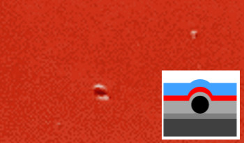
In the automobile industry, a range of defects may occur on automobile exterior surfaces during the external painting process. Such defects may include convex defects stemming from painting on areas where iron powder or dust adheres to the automobile exterior surfaces, and concave defects caused by oil or silicone adhering to the exterior surfaces and repelling the paint [1], as shown in Figure 1. Since defect detection requires significant visual concentration and expertise, efforts are being made to automate this process. In a previous study, Lou and Huang [2] advocated for a proactive approach to quality control utilizing artificial intelligence and engineering principles for addressing complex and uncertain manufacturing processes. They prioritized on-process inspection over post-process inspection and employed hierarchical decision making with fuzzy MIN-MAX algorithms and optimization to evaluate process performance and prevent defects in automotive topcoat applications. Meanwhile, Tanaka et al. [3] concentrated on identifying concave and convex defects on painted surfaces and developed a technique that employs a surface light source and video camera to detect defects and discriminate unevenness. In recent times, research has focused on developing a tunnel-type inspection system [4] (Figure 2) that autonomously detects paint defects, as well as enabling deep-learning-based classification of defect types. Training a deep-learning model for this purpose requires a large dataset consisting of images of parts with paint defects from an automobile exterior that has passed through the inspection system (hereafter referred to as “paint defect images”), as depicted in Figure 3. However, generating such a dataset by capturing images and building individual training models for each customer are expensive and time-consuming processes.

Figure 1.

Schematic and image of paint defects.

Figure 2.

In-line tunnel-type paint defects inspection system esφi [4].

Figure 3.

Example of the paint defect image.

This study proposed a method for generating a learning dataset for each factory by simulating image generation using computer graphics (CG). Figure 4 shows the concept of the proposed method. The shape data of automobile exterior surface paint defects as well as the condition of the inspected object, equipment, and optical arrangement of the factory were simulated to create a CG object (Object A) and the environment (Factory A) that accurately reproduced the defects of the painted automobile exterior surface observed in that factory. The simulation generated a dataset (Dataset A) of images of automobile exterior surface paint defects found in the factory. However, owing to differences in the conditions of the test objects and equipment, a deep-learning model trained on Dataset A cannot accurately classify measured data of defect images from a different factory (Test set B). Therefore, a virtual dataset (Dataset A in B) can be created by generating a reproduction environment of a different factory (Factory B) using CG software and simulating it with Object A’ modified for the different factory test set conditions. The deep-learning model trained on Dataset A in B is expected to classify Test set B with higher accuracy.

Figure 4.

Conceptual diagram of the proposed method.

The efficacy of this method was evaluated by generating two datasets, Dataset A and Dataset A in B, and comparing the classification accuracy in Test set B of deep-learning models trained on Dataset A and Dataset A in B.

Related Works

2.1

Dataset Creation for Deep Learning with CG

In recent years, with research using deep learning becoming popular, many methods for creating training data sets using synthetic data have been proposed [5]. In this section, we introduce some examples. An example of a dataset created using CG is a dataset for a deep-learning model to detect a specific object. Rajpura et al. proposed a method to create a dataset with composite images by rendering packaged foods reproduced in Blender in a virtual environment of a refrigerator to detect packaged foods in a refrigerator [6]. Furthermore, O’Byrne et al. proposed a method to generate synthetic images featuring biofouling in various virtual environments to detect biofouling [7] in marine structures [8]. To avoid privacy issues, several studies have also used CG to build synthetic models of humans when creating datasets containing human face images and videos. Queiroz et al. and Dong et al. proposed pipelines for generating synthetic images of faces using CG [9, 10] In addition, Ragheb et al., De Souza et al., and Varol et al. created a large dataset for human action recognition using CG [11–13].

2.2

Analysis of 3D Data Using 3DCNN

The 3D convolutional neural network (3DCNN) is a neural network architecture proposed by Ji et al. that has been expanded to support three-dimensional input [14]. By performing three-dimensional convolution in the convolution stage, the 3DCNN can compute features from both spatial and temporal dimensions. The 3D convolution is achieved by convolving the 3D kernel into a cube formed by stacking multiple consecutive frames. With this construction, the feature map of the convolutional layer is connected to the previous layer of consecutive frames, enabling the capture of motion information.

The first purpose of using 3DCNN is anomaly detection. Collins et al. constructed a 3DCNN model that detected colon and esophageal cancer with high accuracy by training on hyperspectral image datasets of mucosal tissue in the intracanal regions of the colon and esophagus of patients [15]. Wang et al. also developed a deep autoencoder network for detecting abnormal behavior in surveillance videos, which combines a 3DCNN that encodes short-term temporal and local spatial information and a ConvGRU [16] that encodes long-term temporal and global spatial information [17]. Other examples include fatigue behavior detection for train drivers [18], fall detection for elderly people in a home environment [19], and foul detection within a basketball game [20]. A method for building 3DCNN models to detect videos that exploit deep-faking techniques, which have become a problem in recent years, has also been proposed by Zhang et al. and Wang et al. [21, 22].

Reproduction of Paint Defect Images

This study used Blender [23], an open-source CG software, for generating images of paint defects and datasets. In this section, we present the methodology for generating these images and datasets using Blender.

3.1

Modeling of Defect Shapes

In this study, we generated a dataset consisting of four classes: convex defects, concave defects, fiber defects, and no defects. The shape data for convex and concave defects were generated using the model equation for paint defects by Yoshida et al. [24], while whereas the shape data for fiber defects was based on measured data. The model equations for paint defects used to generate the shape data for convex and concave defects is presented below.

(1)

z = h \cdot e^{- {(\frac{x^{2} + y^{2}}{0.1 \cdot s \cdot d^{2}})}^{s}} .

The parameters of height, diameter, and shape factor are denoted by h, d, and s, respectively. The shape data for convex and concave defects were obtained by generating random values within a predetermined range for each factory. The 3D model geometry resulting from the Eq. (1) computation is shown in Figure 5.

Figure 5.

3D shape of paint defects calculated using the model equation.

3.2

Reproduction of Paint Defects in Factory A

Figure 6 shows the process for reproducing paint defects. First, as depicted in Figure 7, the surface point-cloud data of a paint defect was generated by adding the shape data of the defect at Factory A to the measured shape data of the orange peel, which are minute irregularities appearing on the paint surface. Subsequently, MeshLab [25] software was employed to mesh the point-cloud data by establishing connections between lines and planes. The mesh data of the defect surface were then imported into Blender, where random curvature was introduced to the mesh data to produce variations in the reflection of the light from the inspection device source in the paint defect images. Finally, Object A was created by specifying the material (reflective properties).

Figure 6.

Procedure for reproducing paint defects.

Figure 7.

Conceptual diagram of the procedure for generating a paint defect surface.

3.3

Reproduction of the Environment of Factory A

The creation of Factory A involved the construction of a virtual environment based on the optical arrangement and conditions present in the real-world Factory A. As depicted in Figure 8, this involved the placement of a camera and an arch-shaped light source to simulate the real-world environment. Additionally, Object A, generated using the methodology outlined in Section 3.1, was placed within Factory A and given horizontal motion animation. A 101 × 101 × 33 (frame) image of the defect was produced by limiting the render area to the region surrounding the paint defect.

Figure 8.

Optical arrangement.

Figure 9 compares the simulated image in Dataset A generated using the above method with an image captured in a real environment. To demonstrate the similarity between the measured and generated images, a subjective evaluation experiment was conducted where 9 students evaluated three types of automotive paint defects: concave, convex, and fiber. The students were presented with 10 simulated videos generated from the measured videos of concave, convex, and fiber defects, respectively, and asked to evaluate each defect individually. A five-level evaluation index was used in the evaluation process as shown in Figure 10, with higher numbers indicating greater similarity. The evaluation results for concave, convex, and fiber defects are shown in Figures 11–13. On the vertical axis is the evaluation value and on the horizontal axis is the number of the presented defect movies. The average mean evaluation scores for concave, convex, and fiber defects were 3.36, 3.35, and 3.25 points, respectively. The particularly low evaluation score for fiber defects is thought to be due to the variation in the shape of the fibers falling on the surface of the coating and the differences between factories.

Figure 9.

Comparison of captured and simulated images (right: captured, left: simulated).

Figure 10.

Five-level evaluation index of subjective evaluation experiments.

Figure 11.

Subjective evaluation results for concave defects.

Figure 12.

Subjective evaluation results for convex defects.

Figure 13.

Subjective evaluation results for fiber defects.

Although the student evaluation results were not ideal based on the average from the questionnaire, the fact that the evaluations by experts showed a remarkable similarity to the images captured confirmed the validity of the generated images.

3.4

Change of Environmental Conditions to Factory B

Table I shows the differences in the equipment and test object conditions at each factory. As shown in Figure 14, simulations can generate paint defect images with varying appearances by changing these conditions despite possessing similar defect shape data.

Figure 14.

Comparison of simulation results (Right: Factory A, Left: Factory B).

Table I.

Differences between factories.

Category	Item	Factory A
Equipment	Focal length (mm)	9, 12.5, 16
	F number	7
	Number of pixels (px)	4097 × 3000
	Pixel sixe (μm)	3.45
	Object distance (mm)	600–1600
	Shooting pitch	4
	(mm/frame)
Test object	Body shape	Flat surfaces: 70%
		Curved surfaces: 30%
	Level of orange peel	Good
		(amplitude 1.4–5.0x)
	Distribution of	Black and white only
	paint colors
Category	Item	Factory B
Equipment	Focal length (mm)	16, 25, 35
	F number	7
	Number of pixels (px)	4096 × 2168
	Pixel size (μm)	3.45
	Object disance (mm)	600–1600
	Shooting pitch	2.5
	(mm/frame)
Test object	Body shape	Flat surfaces: 30%
		Curved surfaces: 70%
	Level of orange peel	Bad
		(amplitude 1.4–15.0x)
	Distribution of	Black and white
	paint colors	plus solid colors

The procedure for generating Dataset A in B, a virtual dataset for Factory B, is described as follows. First, the shape data of paint defects used to generate Dataset A was prepared. Subsequently, the defect shape data of Factory A was used to generate a defect surface CG object; Object A’ that reproduces the test object conditions of Factory B. Next, Factory B, which reproduced the equipment conditions of Factory B, was generated. Finally, by placing Object A’ in Factory B and executing a simulation, Dataset A in B was generated.

Comparison of Classification Accuracy using 3DCNN

In this study, we used 3DCNN to compare the classification accuracy of Test set B when trained on two datasets. As there was no Test set B containing captured images in this study, we generated Test set B through simulation using Blender. Table II shows the number of data samples per class included in each dataset.

Table II.

Number of data samples for each class in datasets.

Data set A		Data set A in B		Test set B

Class	Number	Class	Number	Class	Number
	of data		of data		of data
Convex	900	Convex	900	Convex	840
Concave	240	Concave	240	Concave	324
Fiber	60	Fiber	60	Fiber	36
No defects	240	No defects	240	No defects	240
Total	1440	Total	1440	Total	1440

4.1

Network Architecture

The network architecture of the 3DCNN used in this study is depicted in Figure 15. The input comprises a 33-frame sequence of 101 × 101-pixel paint defect images, with a single channel. The input was subjected to a series of operations, including a 3D convolution layer, 3D maximum value pooling layer, and a dropout layer to alleviate overfitting. Subsequently, it went through additional coupling layers, resulting in the prediction of the probabilities of four classes: convex, concave, fiber, and no defects.

Figure 15.

Network architecture.

4.2

Training

The 3DCNN model was trained on Dataset A (Model A) and Dataset A in B (Model A in B), which were divided into 80% for training and 20% for validation according to Pareto’s law [26]. The 80/20 split ratio is one of the most common ratios in the deep-learning field [27, 28]. The training was performed for 40 epochs using the hardware environment specified in Table III, with the optimization function set to Adam, learning rate of 0.0001, and batch size of 8. The learning process took approximately 16 minutes. Figure 16 shows the changes in losses during the learning process.

Figure 16.

Changes in loss during the learning process (Right: Model A, Left: Model A in B).

Table III.

Hardware environment.

CPU	Intel®Xeon (R) Silver 4116 CPU @ 2.10 GHz × 48
RAM	93G DDR4
GPU	NVDIA GeForce RTX 2080 Ti × 4, Quadro P400

4.3

Comparison of Classification Accuracy

We compared the detection results of both models using four indicators: precision, true positive rate (TPR), F1 score, and accuracy. We further evaluated them using the area under the curve (AUC) indicator derived from the receiver operating characteristic (ROC) curve. AUC measures the classification performance and diagnosis rules that are widely used [29–31].

Table IV shows the confusion matrix, where true positive (TP) means that a positive sample was correctly identified, true negative (TN) means that a negative sample was correctly identified, false positive (FP) means that a negative sample was incorrectly identified as positive, and false negative (FN) means that a positive sample was incorrectly identified as negative.

Table IV.

Confusion matrix.

		Predicted value
		Positive	Negative
Correct value	Positive	TP	FN
	Positive	True positive	False negative
	Negative	FP	TN
	Negative	False positive	True negative

Precision is defined as in Eq. (2) and indicates the percentage of TP samples among the samples identified as positive.

(2)

Precision = \frac{T P}{T P + F P} .

TPR is defined as in Eq. (3) and indicates the percentage of positive samples in the data that are correctly discriminated.

(3)

T P R = \frac{T P}{T P + F N} .

The precision of TPR and repeatability alone do not provide a good assessment of model performance. Therefore, we introduced the F1 score to consider fit and reproducibility together. Its definition is shown in Eq. (4).

(4)

F 1 = 2 \frac{Precision \cdot T P R}{Precision + T P R} .

Accuracy is generally used to evaluate the global accuracy of a model, which contains insufficient information and does not provide a comprehensive evaluation of the performance of the model. It is defined as in Eq. (5).

(5)

Accuracy = \frac{T P + T N}{T P + T N + F P + F N} .

Tables V and VI show the confusion matrices for Model A and Model A in B. Comparing the tables, Model A in B detects concave and convex defects more accurately than Model A. This shows that Model A in B more accurately identifies these defects. To further quantify and evaluate the performance of both models, the accuracy evaluation results from the confusion matrices of both models are presented in Tables VII and VIII. The tables show that Model A in B outperforms Model A in all evaluation indices except TPR for fiber defects and no defects. The relatively low TPR for fiber defects may be due to the difficult nature of accurately classifying fiber defects, which vary in shape between factories.

Table V.

Confusion matrix of Model A.

Model A

		Predicted
		Convex	Concave	Fiber	No defects
True	Convex	751	21	7	61
	Concave	17	256	14	37
	Fiber	1	2	30	3
	No defects	0	0	0	240

Table VI.

Confusion matrix of Model A in B.

Model A in B

		Predicted
		Convex	Concave	Fiber	No defects
True	Convex	827	5	0	8
	Concave	5	319	0	0
	Fiber	5	3	28	0
	No defects	0	0	0	240

Table VII.

Accuracy evaluation results for Model A.

Class	Convex	Concave	Fiber	No defects
Precision	0.977	0.918	0.588	0.704
TPR	0.894	0.790	0.833	1.00
F1 Score	0.933	0.849	0.690	0.826
Accuracy	0.886

Table VIII.

Accuracy evaluation results for Model A in B.

Class	Convex	Concave	Fiber	No defects
Precision	0.988	0.976	1.000	0.968
TPR	0.985	0.985	0.778	1.00
F1 Score	0.986	0.980	0.875	0.984
Accuracy	0.982

Figures 17 and 18 depict the ROC curves obtained from Model A and Model A in B, respectively. The horizontal and vertical axes of the ROC curve represent TPR and FPR, respectively. FPR signifies the percentage of negative samples misclassified as positive. Its definition is shown in Eq. (6).

(6)

F P R = \frac{F P}{T N + F P} .

The upward curvature in both cases signifies that these models achieved low FPR while maintaining high TPR, indicating their robust performance. This is indicative of the ability of the models to accurately predict positive samples while minimizing misclassifications of negative samples as positive. Notably, the ROC curve of Model A in B exhibits higher elevation compared to that of Model A, suggesting superior discriminative power. A higher ROC curve elevation signifies that Model A in B achieved a more balanced classification performance, making it better suited for defect detection in Factory B.

Figure 17.

Receiver operating characteristic (ROC) curve of Model A.

Figure 18.

Receiver operating characteristic (ROC) curve of Model A in B.

The AUC values, as presented in Table IX, further support the performance evaluation. AUC values closer to 1.0 indicate better model performance, close to the ideal model with perfect predictive ability. Comparing both models, Model A in B outperforms Model A in all defect classifications, demonstrating its superiority. The comparisons collectively corroborate the higher accuracy of Model A in B over Model A, thereby affirming the efficacy of the proposed method.

Table IX.

AUC comparison of two models.

Model A		Model A in B

Class	AUC	Class	AUC
Convex	0.957	Convex	0.995
Concave	0.964	Concave	0.999
Fiber	0.942	Fiber	0.988
No defects	0.961	No defects	0.997

Summary and Future Work

In this paper, we presented a novel method for generating factory-specific datasets for paint-defect classification of automotive exteriors. By using Blender to simulate paint defects and the factory environment, our approach eliminates the need for new data collection and thus provides a cost-effective and efficient solution. Experimental results show a significant improvement in test set classification accuracy, supporting the effectiveness of the proposed method. The ability to generate factory-specific datasets considers the variation in paint defects across different factories and improves the performance of the model for real-world applications. To the best of our knowledge, no similar study has used the proposed method, thus proving the novelty and uniqueness of our contribution, as this study is pioneering in its approach. Our study lays the foundation to facilitate the practice of defect classification in the automotive industry and optimize the quality control process.

Future work includes superimposing paint defects on the automobile model and mapping measured values to material parameters to generate simulations that more closely resemble inspections under real-world conditions.

References

1Nippon Kako Toryo Co., Ltd., “Nippon Kakoh Paint”. (accessed 16 January)

2LouH. H.HuangY. L.2003Hierarchical decision making for proactive quality control: system development for defect reduction in automotive coating operationsEng. Appl. Artif. Intell.16237250237–5010.1016/S0952-1976(03)00060-5

3TanakaK.ShinbaraY.IkedaH.YamadaN.KibaH.SasanishiK.1994Automated inspection method for painted surfacesTrans. Jap. Soc. Mech. Eng.60866873866–73

4Konica Minolita Japan, INC., “Inline Tunnel Type Coating Defect Inspection System esφi | KONICA MINOLITA JAPAN, INC.- Powered byIPROS CORPORATION.” (accessed 16 January)

5NikolenkoS. I.Synthetic Data for Deep Learning.2021SpringerCham174

6RajpuraP. S.HegdeR. S.BojinovH.Object Detection Using Deep CNNs Trained on Synthetic Images. arXiv:abs/1706.06782 (2017)

7KazuhisaT2009Biofouling in seawater reverse osmosis desalination plantBull. Soc. Sea Water Sci., Jpn.63303306303–6

8O’ByrneM.PakrashiV.SchoefsF.GhoshB.2018Semantic segmentation of underwater imagery using deep networks trained on synthetic imageryJ. Marine Sci. Eng.69310.3390/jmse6030093

9QueirozR.CohenM.MoreiraJ. L.BraunA.Jacques JuniorJ. C.MusseS. R.2010Generating facial ground truth with synthetic faces2010 23rd SIBGRAPI Conf. on Graphics253125–31IEEEPiscataway, NJ10.1109/SIBGRAPI.2010.12

10DongY.LinM.YueJ.ShiL.2019A low-cost photorealistic CG dataset rendering pipeline for facial landmark localizationMultimedia Tools Appl.78223972242022397–42010.1007/s11042-019-7516-5

11RaghebH.VelastinS.RemagninoP.EllisT.2008Vihasi: virtual human action silhouette data for the performance evaluation of silhouette-based action recognition methods2008 2nd ACM/IEEE Int’l. Conf. on Distributed Smart Cameras1101–10IEEEPiscataway, NJ10.1109/ICDSC.2008.4635730

12De SouzaC. R.GaidonA.CabonY.L’opezA. M.2017Procedural generation of videos to train deep action recognition networks2017 IEEE Conf. on Computer Vision and Pattern Recognition (CVPR)259426042594–604IEEEPiscataway, NJ10.1109/CVPR.2017.278

13VarolG.RomeroJ.MartinX.MahmoodN.BlackM. J.LaptevI.SchmidC.2017Learning from synthetic humans2017 IEEE Conf. on Computer Vision and Pattern Recognition (CVPR)462746354627–35IEEEPiscataway, NJ10.1109/CVPR.2017.492

14JiS.XuW.YangM.YuK.20133D Convolutional neural networks for human action recognitionIEEE Trans. Pattern Anal. Mach. Intell.35221231221–3110.1109/TPAMI.2012.59

15CollinsT.MaktabiM.BarberioM.BencteuxV.Jansen-WinkelnB.ChalopinC.MarescauxJ.HostettlerA.DianaM.GockelI.2021Automatic recognition of colon and esophagogastric cancer with machine learning and hyperspectral imagingDiagnostics11181010.3390/diagnostics11101810

16BallasN.YaoL.PalC.CourvilleA.2016Delving deeper into convolutional networks for learning video representationsInt’l. Conf. on Learning Representations (ICLR)1111–1110.48550/arXiv.1511.06432

17WangX.XieW.SongJ.2018Learning spatiotemporal features with 3DCNN and ConvGRU for video anomaly detection2018 14th IEEE Int’l. Conf. on Signal Processing (ICSP)474479474–9IEEEPiscataway, NJ10.1109/ICSP.2018.8652354

18LiuY.ZhangT.LiZ.20193DCNN-based real-time driver fatigue behavior detection in urban rail transitIEEE Access7144648144662144648–6210.1109/ACCESS.2019.2945136

19HsiehY. Z.JengY. L.2018Development of home intelligent fall detection IoT system based on feedback optical flow convolutional neural networkIEEE Access6604860576048–5710.1109/ACCESS.2017.2771389

20LinC. H.TsaiM. Y.ChouP. Y.2021A lightweight fine-grained action recognition network for basketball foul detection2021 IEEE Int’l. Conf. on Consumer Electronics-Taiwan (ICCE-TW)121–2IEEEPiscataway, NJ10.1109/ICCE-TW52618.2021.9602903

21ZhangD.LiC.LinF.ZengD.GeS.2021Detecting deepfake videos with temporal dropout 3DCNNProc. 13th Int’l. Joint Conf. on Artificial Intelligence (IJCAI-21)128812941288–94IEEEPiscataway, NJ10.24963/ijcai.2021/178

22WangY.DantchevaA.2020A video is worth more than 1000 lies. Comparing 3DCNN approaches for detecting deepfakes2020 15th IEEE Int’l. Conf. on Automatic Face and Gesture Recognition (FG 2020)515519515–9IEEEPiscataway, NJ10.1109/FG47880.2020.00089

23Blender. Blender. https://www.blender.org/. (accessed 16 January)

24YoshidaR.NagaiY.KashiwabaraM.“A study of “scales” and “defect samples” for coating defect inspection,” 37th Annual Conf. on Paint and Coating Research (2022)

25MeshLab. MeshLab. https://www.meshlab.net/. (accessed 16 January)

26Dunford.R.SuQ.TamangE.2014The pareto principlePlymouth Stud. Sci.7140148140–8

27JainG.MittalD.TakurD.MittalM. K.2020A deep learning approach to detect COVID-19 coronavirus with X-ray imagesBiocybern. Biomed. Eng.40139114051391–40510.1016/j.bbe.2020.08.008

28Abdelaziz IsmaelS.MohammedA.HefnyH.2020An enhanced deep learning approach for brain cancer MRI images classification using residual networksArtif. Intell. Med.10210177910.1016/j.artmed.2019.101779

29BradleyA. P.1997The use of the area under the ROC curve in the evaluation of machine learning algorithmsPattern Recognit.30114511591145–5910.1016/S0031-3203(96)00142-2

30HandD. J.TillR. J.2001A simple generalisation of the area under the roc curve for multiple class classification problemsMach. Learn.45171186171–8610.1023/A:1010920819831

31HanleyJ. A.1989Receiver operating characteristic (ROC) methodology: the state of the artCrit. Rev. Diagn Imag.29307335307–35