Back to articles
CIC34 (2026)
Volume: 9 | Article ID: 000402
Image
Bridging Physical Additivity and Simultaneous Contrast: An Analysis of Nonlinearities in Color Appearance in Optical See-Through Augmented Reality
  DOI :  10.2352/J.Percept.Imaging.2026.9.000402  Published Online :  October 2026
Abstract
Abstract

The perceived color in optical see-through augmented reality (AR) deviates from physical additivity, but the driving factors and their interactions remain poorly understood. The authors conducted four psychophysical color-matching experiments manipulating seven factors including stimulus size, viewing mode, starting point, and presentation medium. A generalized linear mixed-effects model analysis of the coordinate-wise differences in CIECAM16-UCS space revealed stimulus size as the strongest predictor. Reducing the stimulus size—which increases the relative area of the chromatic surround—produced shifts that tended to be opposite to the background chromaticity, consistent with classical simultaneous contrast. The viewing mode and presentation medium had small effects concentrated on the blue–yellow axis, whereas the starting point produced a small procedural shift across all axes. The linear additive model showed limitations: nonlinear deviations were confined to specific targets where chromatic induction was strongest. These findings suggest that background discounting in AR largely reflects low-level simultaneous contrast, complementing higher-level accounts such as layer scissioning.

Supplementary Material
Subject Areas :
Views 24
Downloads 6
 articleview.views 24
 articleview.downloads 6
  Cite this article 

Wei Li, Midori Tanaka, Takahiko Horiuchi, "Bridging Physical Additivity and Simultaneous Contrast: An Analysis of Nonlinearities in Color Appearance in Optical See-Through Augmented Reality"  in Journal of Perceptual Imaging,  2026,  pp 1 - 14,  https://doi.org/10.2352/J.Percept.Imaging.2026.9.000402

 Copy citation
  Copyright statement 
This work is licensed under the Creative Commons Attribution 4.0 International License. To view a copy of this license, visit http://creativecommons.org/licenses/by/4.0/.
  Article timeline 
  • received May 2026
  • accepted August 2026
  • PublishedOctober 2026

Preprint submitted to:
jpi
Journal of Perceptual Imaging
J. Percept. Imaging
J. Percept. Imaging
2575-8144
Society for Imaging Science and Technology
1.
Introduction
In optical see-through augmented reality (OST-AR), the virtual graphics and the physical environment are blended additively on the observer’s retina. From a colorimetric perspective, the tristimulus values of the resulting mixture stimulus are simply the linear sum of the digital foreground emission and the physical background reflection [11]. However, the human visual system is more than a linear photoreceptor. Psychophysical studies demonstrate that the perceived color appearance systematically deviates from this linear additive baseline. Understanding and managing this discrepancy between physical additivity and perceptual color appearance remains a fundamental challenge for color reproduction in AR displays.
To quantify these perceptual deviations, Hassani and Murdoch [16] proposed a weighted foreground–background blending model, often referred to as the αβ model, which describes the perceived tristimulus values as the weighted sum of the foreground (FG) and background (BG):
(1)
XYZeff=αXYZFG+βXYZBG.
In their initial formulation, this weighting was motivated by transparency perception [15]. Subsequent work extended this idea to color layer scissioning [7], suggesting that the visual system decomposes the combined retinal input into an independent virtual layer and a physical background layer. Within this framework, focusing on the foreground corresponds to a reduced background weight (β < 1), a phenomenon referred to as background discounting [26]. Notably, the term “background discounting” has an older origin in classical color science. Walraven [30] used it to describe chromatic induction and receptive field adjustments driven by lateral inhibition—a fundamental low-level, retinal mechanism. This terminological convergence raises the question of whether the background discounting observed in AR reflects a high-level cognitive process (layer scissioning), a low-level simultaneous contrast (SC) effect, or some combination of the two. However, data that could distinguish these accounts are still limited.
The perceived color appearance in OST-AR is shaped by factors spanning multiple levels. At the hardware and photometric level, chromatic adaptation is jointly modulated by ambient illuminance, correlated color temperature (CCT), and display-specific white point and gamut [5, 24]. At the spatial and geometrical levels, depth cues and parallax have been suggested to influence color perception [27], and the degree of spatial alignment between virtual and real content has been shown to substantially modulate perceived color and brightness [23, 26]. Related work has further proposed that the visual system may actively decompose the combined retinal input into independent layers (layer scissioning) [7, 27]. At the level of higher-order perceptual behavior, the complexity and identity of the foreground stimulus have also been found to affect appearance [15, 17, 31].
Despite this progress, existing studies exhibit two notable limitations. First, most investigations have examined individual factors in isolation without systematically exploring interactions among spatial, luminance, and procedural variables. Second, although spatial alignment between the foreground and the background has been identified as a major modulator of perceptual shifts, how other factors—such as stimulus size and viewing mode—affect color appearance under nonaligned, large-background conditions similar to those used by Hassani [15] remains poorly understood.
These observations motivate the current study. We address the question: Under standard nonaligned background conditions, which experimental factors most strongly influence color appearance in additive AR displays, and how do they interact?
To address this question, we conducted four psychophysical color-matching experiments in a controlled AR simulator, systematically manipulating seven factors: viewing mode, stimulus size, aperture presence, foreground spatial offset, starting point, ambient luminance, and presentation medium. We analyzed the matching results in a three-dimensional uniform color space (CIECAM16-UCS), preserving vector directionality. A generalized linear mixed-effects model (GLMM)—a framework highly effective for modeling complex multifactorial interactions and controlling for statistical dependencies in repeated measures—was applied to the pooled dataset, with the response defined as the coordinate-wise difference between the match and the target.
The primary objective of this work is to provide a systematic empirical baseline for color appearance in additive AR displays under chromatic induction. In doing so, we quantify how perceptual deviations from linear additivity depend on the manipulated experimental factors. These results are expected to inform the development of more robust color appearance models for AR environments.
2.
Methods
The experimental paradigm consisted of four experiments designed to systematically investigate the visual contributions and higher-order interactions of multiple environmental and task-related factors. All four experiments utilized a psychophysical color-matching task.
2.1
Apparatus
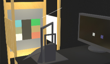
The AR simulator, from our previous experimental setup [23], was housed in a dark room and comprised three main components: a physical background, a digital virtual foreground, and an observation assembly. Figure 1 provides a schematic overview of the apparatus. The physical background pattern was inkjet-printed and mounted at the rear of a custom wooden booth. Two spectrally tunable light sources (Thouslite LEDCube) were positioned at the top and bottom of the booth to provide uniform illumination across the background surface. The virtual foreground was a professional display (EIZO ColorEdge CG277) positioned to match the optical depth plane of the background pattern.
Figure 1.
Schematic diagram of the AR simulator and stimulus layout. (a) Physical apparatus setup, where the display presents the target foreground patch and the adjustable matching foreground patch. (b) Simulated observer’s field of view through the aperture, showing the composite target stimulus (formed by optical superimposition of the foreground patch and the physical chromatic background patch) alongside the adjustable matching stimulus (on the adjacent black patch). The aperture and chin rest (not shown) restricted the field of view at a viewing distance of 1 m. Curtains and input devices are omitted for clarity. Colors are illustrative only. The figure depicts a trial for Target 4 (BG: gray, FG: purple) using a “mid” starting point.
The observation assembly comprised a plate beamsplitter, a magnetic black occlusion panel, an aperture, and a chin rest. Specifically, a plate beamsplitter (Edmund Optics Plate Beamsplitter #68-268, 75:25 reflection/transmission ratio) optically superimposed the self-luminous foreground emission onto the reflective background pattern. Directly behind the beamsplitter, a magnetic black occlusion panel could be deployed to block the light from the background booth for display-only conditions. Progressing toward the observer, a square aperture and a chin rest jointly restricted the observer’s viewpoint and effective field of view. The entire apparatus was enclosed within a black felt curtain to eliminate extraneous visual distractions. The viewing distance was 1 m for both the foreground and the background, with care taken to ensure precise alignment in depth. Observers performed color adjustments via a keyboard placed outside the curtain.
All colorimetric measurements were taken from the observer’s eye position through the beamsplitter using a spectrophotometer (Konica Minolta CS-2000), thereby ensuring accurate measurements of the actually perceived stimuli.
2.1.1
Background Component
Unlike our prior experimental design that relied on explicit geometric registration, this study utilized a Hassani-style background pattern [15] to enable direct comparison with previous paradigms. The background pattern was printed on a paper sheet measuring 54 × 60 cm (all dimensions specified as width × height throughout this paper). Its central 43 × 30 cm region formed a 3 × 3 matrix of nine rectangular color patches, each subtending a visual angle of approximately 8.1∘×5.7∘. The two outer columns contained chromatic patches that served as the target backgrounds, whereas the central column contained three uniform black patches that merged into a seamless black strip, serving as the test backgrounds for the matching task. From top to bottom, the left column comprised blue, gray, and white patches while the right column comprised green, brown, and red patches. The peripheral region surrounding the matrix was filled with a neutral gray background though its visibility was heavily restricted by the aperture.
The background booth accommodated two ambient illumination levels: a high-luminance condition and a low-luminance condition, providing ambient luminances of approximately 31.8 cd/m2 and 7.06 cd/m2 (corresponding to illuminances of 100 lx and 22.2 lx), respectively. The illumination reproduced Hassani’s “cool light”, where the nominal CCT was 4334 K. The spectral power distributions of the light sources were optimized along with the background pattern to reproduce the colorimetric profiles of the background patches used in Hassani’s study although minor chromatic errors remained. The detailed colorimetric coordinates of the background patches (along with their corresponding target mixtures) under both illuminance conditions are reported in Table I.
Table I.
Colorimetric specifications of background patches and their corresponding background–foreground mixtures. The X, Y , and Z values are absolute tristimulus values from which the CIECAM16-UCS coordinates (J  ′, a ′,b ′ values) were computed using the respective mean white points of the two luminance conditions as references. All values are arithmetic means calculated independently within their respective color spaces (CIEXYZ or CIECAM16-UCS).
Target combinationBG colorFG colorAmbient luminanceBG XY ZMixture XY Z BG J  ′a ′b ′ Mixture J  ′a ′b ′
1BlueOrangeLow(1.85, 2.34, 2.70)(6.15, 5.27, 3.96)(69.70, −15.45, −6.68)(92.79, 15.65, 5.23)
High(8.33, 10.44, 11.89)(27.89, 23.84, 18.22)(69.67, −15.99, −7.97)(93.03, 18.42, 4.70)
3GreenGreenLow(1.14, 1.92, 0.70)(1.57, 2.70, 1.50)(64.06, −23.81, 13.82)(72.19, −26.57, 8.83)
High(4.66, 7.69, 2.87)(6.87, 11.57, 6.52)(61.44, −24.56, 14.41)(71.07, −27.74, 8.97)
4GrayPurpleLow(1.63, 1.82, 1.12)(1.93, 2.06, 1.88)(64.28, −5.18, 8.30)(67.38, −3.15, 0.32)
High(7.50, 8.33, 5.08)(8.72, 9.24, 8.51)(64.81, −4.74, 8.92)(67.45, −2.02, −1.20)
6BrownWhiteLow(1.82, 1.89, 0.84)(13.69, 14.04, 22.63)(65.43, −0.86, 12.48)(120.71, 0.10, −29.06)
High(8.30, 8.58, 3.79)(62.38, 63.20, 102.82)(65.79, 0.15, 13.54)(120.74, 3.12, −32.96)
7WhiteBlueLow(6.24, 6.55, 4.12)(7.48, 7.50, 8.29)(97.87, −1.42, 10.16)(101.93, 3.89, −7.96)
High(23.89, 24.90, 15.60)(29.45, 28.82, 35.48)(91.45, 0.35, 10.01)(96.33, 7.46, −13.67)
9RedOrangeLow(1.95, 1.58, 0.65)(4.71, 3.52, 1.44)(62.37, 13.65, 11.92)(82.48, 21.76, 13.38)
High(8.81, 7.18, 2.89)(21.40, 15.88, 6.54)(62.68, 15.46, 13.09)(82.70, 24.81, 14.20)
13GreenRedHigh(5.04, 8.37, 3.11)(14.79, 16.12, 10.27)(63.54, −25.24, 14.69)(81.25, −3.83, 9.33)
19RedGreenHigh(8.71, 7.01, 2.92)(15.07, 16.23, 10.32)(62.19, 16.26, 12.56)(81.48, −2.81, 9.31)
2.1.2
Foreground Component
The foreground display operated at a 10-bit color depth with a native resolution of 2560 × 1440 pixels and a pixel pitch of 0.2331 mm, subtending approximately 0.8 arcmin per pixel. The display was colorimetrically characterized to enable rapid and accurate transformations between CIEXYZ tristimulus values and digital RGB values with minimal errors. To align with the two illuminance conditions, the peak display luminance was manually toggled via the monitor’s physical hardware controls to either 300 cd/m2 or 75 cd/m2, with the display characterization model updated to reflect the corresponding luminance setting. This adjustment maximized the display’s usable dynamic range under both illuminance conditions, preventing quantization errors and ensuring finer control during color matching.
Across all experiments, foreground targets and background patches were generally paired one to one using coordinates from the previous literature [15]. In Experiment 1, two backgrounds were additionally paired with a second foreground to investigate background chromatic induction. The target colors were defined by the tristimulus values of the additive mixture, representing the physical sum of the background and foreground (XY Zmixture = XY ZFG + XY ZBG). During the trials, the control program calculated the required digital RGB values based on the measured background tristimulus values and the characterization profile scaled to the selected luminance level. This generated a virtual foreground target stimulus that was spatially nested within the boundary of the background patch. Concurrently, an identical-sized adjustable matching stimulus was displayed on the adjacent black patch in the central column.
2.1.3
Matching Software and Procedure
The psychophysical matching program was implemented in MATLAB using the Psychophysics Toolbox Version 3 [20]. Observers independently manipulated chroma, hue, and lightness within the CIELCH color space. The program provided interactive functionalities allowing observers to toggle between the current matching state and the initial starting color coordinates, to save and recall up to three intermediate matching states, and to confirm the final match to advance the trial.
The white patch located in the lower-left corner of the matrix was initially selected as the reference white point for the CIELCH transformation, but it was noticeably yellowish. This caused the color trajectory during chroma adjustments to deviate from subjective neutral white, introducing unintended hue shifts and increasing task difficulty. To address this, a white-point adjustment mode was introduced to customize the color space transformation for each individual and to quantify the observer’s actual chromatic adaptation state under the current ambient conditions. Subsequent statistical analysis confirmed that individual white-point adjustment did not exert a significant effect on the final matching coordinates (see Appendix A.5, Supplementary Material). Full procedural details and session coverage are provided in Appendix A.1 and Table B1 (Supplementary Material).
2.2
Experimental Design
Within each experiment, trials were organized into distinct phases primarily dictated by the physical constraints of toggling certain environmental hardware (e.g., swapping presentation media or modifying ambient luminance). Within each phase, the presentation order of target colors was randomly shuffled to ensure that no identical color target appeared consecutively. Each phase evaluated a predefined set of target colors, with each target repeated twice.
The multifactorial design isolated and evaluated seven environmental, spatial, and procedural factors across the four experiments. Specifically, Experiment 1 primarily investigated the effects of stimulus size and viewing mode (binocular or monocular viewing); Experiment 2 examined the presence of aperture, foreground spatial offset (the presence of a minor positional change of the foreground patch), and the starting point (the initial color configuration of the test patch); Experiment 3 focused on ambient luminance levels (the interior luminance of the booth in AR or its digitally simulated counterpart on screen) and the presentation medium (AR simulator or display-only); and Experiment 4 investigated the starting point and presentation medium. Table II summarizes the manipulated factors, their levels, and the variable names used in subsequent statistical modeling along with operational descriptions clarifying the technical and perceptual definitions of complex procedural factors.
Table II.
Experimental factors, levels, and operational descriptions (bold text indicates the default baseline level used across experiments).
FactorVariableLevelsDescription
Viewing modeview_modeMonocular, binocularMonocular trials used a gauze patch over the nondominant eye
Stimulus sizestim_sizeSmall (4 × 4 cm or 2.3∘×2.3∘), large (13.5 × 9.5 cm or 7.7∘×5.4∘)Applies identically to both target and test patches
Aperture presenceaperturePresent, absentWhen absent, the aperture is removed for a wider view of the booth
Foreground spatial offsetfg_offsetAligned,
offset (3∘ rotation + 12 mm or 40 ′ horizontal)
Target FG shifts 12 mm or 40 ′ horizontally away from central column
Starting pointstart_pointLow (RGBtest = RGBtarget),
mid (XY Ztest = XY Ztarget),
high (2 ⋅ XY Zmid − XY Zlow)
Initial test patch color
Mid matches target mixture XY Z; low uses target foreground digital RGB values on black background (perceptually darker); high is mathematically extrapolated using the values from the mid and low levels to be brighter
Ambient luminanceambient_lumLow (≈7.06 cd/m2), high (≈31.8 cd/m2)Interior luminance of the background booth or the digitally simulated background luminance rendered on screen
Presentation mediummediumAR, display-onlyAR uses the optical mixture. Display-only uses a closed occlusion panel and digitally reproduces the background pattern on screen
Specifically, for the display-only medium condition, the physical background pattern was reproduced on the screen by sampling the measured tristimulus values at the four corners of each physical patch and applying a linear RGB gradient within each patch boundary to preserve a natural paper-like appearance. The surrounding region outside the patches was rendered a uniform neutral gray.
An aggregate of eight foreground–background target combinations (target_id) was evaluated. Six combinations, labeled 1, 3, 4, 6, 7, and 9 according to their spatial layout on the background pattern (ordered top to bottom, left to right), mapped six background patches to six distinct intended target colors and were shared across multiple experiments. Two additional combinations, labeled 13 and 19, were evaluated exclusively in Experiment 1. Specifically, Target 13 features a red foreground on a green background while Target 19 features a green foreground on a red background. These two targets were designed to have the same intended target chromaticities, thereby allowing a direct probe into background chromatic effects. The complete colorimetric specifications of all background patches and their corresponding target mixtures are summarized in Table I.
2.3
Observers
A total of 12 observers (aged 22–32 years, three females and nine males) participated in the study. Each experiment involved eight participants, meaning that individual observers completed between one and four experiments. All observers passed the Ishihara test to confirm normal color vision, and all had prior experience with general color-matching experiments.
This study was conducted in accordance with the Declaration of Helsinki. Given the noninvasive nature of these psychophysical procedures, which involved no greater risk than everyday visual activities, formal ethics approval was not required under institutional guidelines. All observers provided written informed consent prior to participation and were debriefed after completing the sessions.
2.4
Procedure
Prior to each experimental session, the experimenter preheated the background light sources for at least 1 h and the display for at least 30 min. Upon entering the dark room, observers adapted for at least 5 min while the experimenter explained the general workflow, trial counts, and control mechanisms. Observers were then allowed to practice with the keyboard freely. Following adaptation, observers completed the white-point adjustment (for sessions where this feature was active) and initiated the matching trials at their own discretion. Observers were permitted to take breaks or leave the room at any time, provided that they underwent readaptation upon returning.
Experiments 3 and 4 involved switching between AR and display-only media. Observers experiencing this transition for the first time were requested to look away during the phase switch to keep them unaware of the medium transition. In the follow-up experiment, they were directly notified of the change. After completion of the psychophysical tasks, a validation program read the recorded RGB values and reproduced the matched patches at their identical positions and sizes. The corresponding XY Z tristimulus values were then systematically measured using the spectrophotometer while the background occlusion board was closed to ensure radiometric accuracy. The display was verified to be sufficiently stable to allow these measurements to be conducted following the completion of each observer’s experimental session.
The four experiments were not executed in a strict chronological sequence. Individual white-point adjustments were performed by three participants in Experiment 1, six participants in Experiment 2, and all participants in Experiments 3 and 4. Regarding medium transition, all observers were completely naïve to the purpose and existence of the change during their first exposure (either in Experiment 3 or 4). In the subsequent follow-up experiment, observers were explicitly notified of the transition as part of the experimental protocol, resulting in one observer in Experiment 3 and seven observers in Experiment 4 being aware of the display-only medium during their respective second test sessions.
2.5
Data Preparation
The recorded measurements were transformed into a uniform color space combining the CIECAM16 color appearance model [18] and the CAM16-UCS conversion algorithm [22], designated CIECAM16-UCS throughout this paper. Reference white points for high- (31.8 cd/m2) and low-luminance (7.06 cd/m2) conditions were derived from mean observer-adjusted chromaticity coordinates (Appendix A.2, Supplementary Material). Because only the nine color patches within the central matrix were visible during most of the trials, the relative background luminance Y b was set at their mean luminance value of 26.28, and the viewing condition parameter was specified as “dim” for the CIECAM16 model configuration.
To eliminate obvious procedural matching blunders, multivariate outlier removal [14] was performed using Mahalanobis distance within subgroups (8 observers × 2 repetitions per target combination). This procedure identified and excluded 12 extreme outliers out of 1088 total observations (Appendix A.3, Supplementary Material). To resolve the unbalanced design in Experiment 3 caused by procedural constraints, corresponding observations were supplemented from Experiments 1 and 2 during preliminary factor screening (Appendix A.4, Supplementary Material).
2.6
Statistical Analysis
The statistical analysis began with descriptive metrics to evaluate empirical matching precision and target deviation, followed by a structured GLMM framework to isolate independent factor effects and assess their relative contributions to perceptual color shifts.
2.6.1
Descriptive Evaluation Metrics
Matching precision and overall perceptual bias were quantified using mean Euclidean distance from the mean (MEDM) and mean Euclidean distance from the target (MEDT) within each subgroup in CIECAM16-UCS:
(2)
MEDM =1N∑i=1N∥xi−x¯∥2
(3)
MEDT =1N∑i=1N∥xi−xtarget∥2,
where xi represents the matched coordinate vector of trial i, x¯ is the condition-wise arithmetic mean, and xtarget denotes the physical target coordinate vector.
2.6.2
GLMM Specifications
The cleaned dataset was analyzed in R (version 4.5.2) [28] using the glmmTMB package [4]. A linear mixed-effects model [25] provides a regression-based framework capable of simultaneous modeling of fixed and random effects, making it highly effective for analyzing unbalanced data structures containing repeated measures while controlling for random variations across individual observers. Extending this framework, GLMM [3] directly accommodates high-dimensional datasets and permits conditional response distributions to follow non-normal profiles while explicitly supporting the configuration of heteroscedastic structures. Although less conventional in standard color science, this statistical approach is well suited for the complexities of our psychophysics tasks. Specifically, it allows us to systematically control for interobserver adjustment preferences as random effects while analyzing repeated-measures data. Furthermore, unlike the traditional analysis of variance, the GLMM framework gracefully handles the unbalanced data structures resulting from our multifactorial design and enables the configuration of heteroscedastic error distributions directly aligned with human color-matching volatility.
The statistical analysis focused on seven experimental factors—viewing mode, stimulus size, aperture presence, foreground spatial offset, starting point, ambient luminance, and presentation medium—along with two specific interactions: between the viewing mode and the stimulus size, and between the starting point and the presentation medium. The response variable was defined as the colorimetric difference vector (Diff), calculated as the matched color minus the intended target color within the CIECAM16-UCS space. To model the three-dimensional color coordinates, the data was converted into a long format, introducing a new fixed factor, coordinate axis (axis). All explanatory variables, including both fixed and random effects, were treated as categorical factors. The random-effects structure with observers as the grouping variable was specified as (0 + axis | observer) to account for interobserver variability across the three perceptual dimensions. While structurally specified as random slopes, this configuration functionally assigns distinct but correlated random intercepts to each axis.
The dispersion model was specified as ∼axis * target_id, which allowed conditional residual variances to be heteroscedastically distributed across different target colors and coordinate axes. The conditional response distribution was specified using t_family() to minimize the influence of extreme values and enhance the structural robustness of the model estimates against influential outliers and heavy-tailed residual distributions.
2.6.3
Analytical Strategy and Model Selection
To establish a unified and directly comparable hierarchy of all experimental factors, our modeling strategy adopted a two-stage approach: we first screened for significant predictors within individual experiments and subsequently consolidated these key factors into a single pooled model.
In the initial screening stage, model selection followed a top-down refinement process starting from a full multivariate GLMM within each of the four experiments. Candidate models incorporating experimental factors of interest, their mutual interactions, and their interactions with the control variables (coordinate axis and target combination) were evaluated using standard maximum likelihood estimation, and the model yielding the minimum corrected Akaike Information Criterion (AICc) [29] was selected as the optimal structure, with lower values indicating a superior balance between model fit and parsimony. During this stage, candidate dispersion formulas were also evaluated, with ∼axis * target_id selected as it maximized the reproduction of empirical variance characteristics while maintaining strict model convergence.
In the second stage, the significant predictors identified from individual experiments were consolidated into a unified formula and applied to the pooled dataset. Top-down AICc comparisons supported retaining (0 + axis | observer) as the optimal random-effects structure without an interexperiment random intercept. Secondary procedural factors—specifically white-point adjustment status (wp_adjusted) and observer awareness of the display medium (disp_aware)—were evaluated and excluded due to nonsignificant contributions, confirming that perceptual matching was robust against white-point adjustment and medium awareness (see Appendix A.5, Supplementary Material for selection details).
Final parameter estimates for the consolidated pooled model were computed using restricted maximum likelihood to ensure unbiasedness and robustness [25]. Pooling the data across experiments provides two methodological advantages: first, integrating conditions with shared factor levels maximizes the available control data, thereby enhancing statistical power and estimation stability; second, a single consolidated model enables a direct, quantitative comparison of the relative effect sizes across all significant factors within a unified framework.
2.6.4
Statistical Inference and Model Evaluation
Model adequacy and distributional assumptions were first evaluated through standard diagnostic procedures. Residual distribution adequacy, conditional dispersion, and potential outliers were verified using DHARMa-based diagnostics. Multicollinearity among predictors was assessed using variance inflation factors. Model precision and variance partitioning were additionally summarized using mean absolute errors (MAEs) across coordinate axes, observer random-effects standard deviations, and the interclass correlation coefficient (ICC).
Upon confirming model validity, the statistical contribution of experimental factors in the final pooled model was evaluated using Type III Wald χ2 tests. To interpret significant main effects, estimated marginal means (EMMs) [21] were computed for all unique combinations of the significant factors. To quantify the direction and the magnitude of each factor’s effect, pairwise contrasts were additionally computed under standardized reference conditions: for each factor, the levels being compared were evaluated while holding the remaining factors at their default baseline levels.
3.
Results
3.1
Raw Data Overview
The CIECAM16-UCS coordinates were computed using observer-adjusted, condition-specific white points (established in Section 2.5; detailed in Appendix A.5, Supplementary Material). Based on these, observer precision (MEDM) and target deviation (MEDT) were quantified across Experiments 1–4 to establish baseline response quality.
In Experiment 1, raw matches showed the highest precision (MEDM = 2.61) and smallest target shifts (MEDT = 4.36), driven by the large stimulus size condition (MEDM = 2.05, MEDT = 3.48). In Experiments 2–4 (conducted under small-stimulus conditions), observer variability (MEDM = 4.39–4.60) and target shifts (MEDT = 6.19–7.85) were larger but more consistent. Across targets, Target 4 (BG: gray, FG: purple) exhibited the largest shift (MEDT = 11.53) whereas Targets 9, 13, and 19 maintained higher fidelity (MEDT = 3.13–3.46).
In addition, the raw matching distribution reveals a subtle procedural anchoring effect. As demonstrated in Figure 2, adjustments starting from “low” starting points systematically fall between the mean match from the “mid” condition and the starting point itself. The displacement between matches from the “low” and “mid” starting points ranges from ΔE  ′ = 0.26 to 1.82 across targets.
Figure 2.
Procedural anchoring effect across low starting points. Symbols are defined in the figure legend. Points represent mean matches under corresponding starting colors, color-coded by target combination. Adjustments starting from the “low” condition systematically fall between the “mid” mean match and the starting point.
These preliminary observations from the raw data revealed two empirical tendencies that motivated the subsequent GLMM analysis. First, observer variability and target deviation were substantially larger under the small-stimulus conditions than under the large-stimulus conditions, indicating that stimulus size strongly influenced matching performance. Second, matches initiated from the low starting point consistently remained closer to their initial values than those from the mid starting point, suggesting a procedural anchoring tendency (Fig. 2).
Although these descriptive observations provide an intuitive overview of the data, they do not isolate the individual contributions of the multiple experimental factors because of the unbalanced factorial design and the overlap among experiments. Therefore, a multivariate GLMM framework was implemented using signed coordinate differences as responses to quantify the independent effects of each predictor.
3.2
Model Selection Outcomes and Validation
Following the two-stage model selection strategy outlined in Section 2.6.3, top-down refinement was first applied within each individual experiment dataset to identify statistically significant predictors and interaction terms. Model comparison based on AICc yielded the following optimal fixed-effects specifications for the four experiments (with detailed selection tables provided in Appendix Tables B3.1–B3.4, Supplementary Material):
Experiment 1: Diff  ∼ axis * (view_mode + stim_size * target_id)
Experiment 2: Diff  ∼ axis * (start_point + target_id)
Experiment 3: Diff  ∼ axis * (ambient_lum * target_id + medium)
Experiment 4: Diff  ∼ axis * (start_point + target_id) + medium
Across the pooled dataset (comprising 1076 trials, corresponding to 3228 long-format observations across the three coordinate axes after outlier removal), the significant predictors identified from the individual experiments were consolidated into a single pooled framework. The final pooled model retained viewing mode, stimulus size, ambient luminance, starting point, and presentation medium as the primary predictors, while aperture presence, foreground offset, and the aforementioned interactions were excluded due to lack of statistical contribution. The fixed-effects formula for the consolidated pooled model is specified as follows (Appendix Table B3.5, Supplementary Material):
Diff   ∼  axis  *  (target_id  *  (stim_size  +  ambient_lum) +  start_point  +  view_mode  +  medium)
In this specification, color-related factors interacting with target combinations are placed first within the formula. All individual and pooled models maintained the baseline random-effects structure (0 + axis | observer) and conditional dispersion model ∼axis * target_id defined in Section 2.6.2. Fitting this consolidated framework captured the systematic underlying perceptual patterns while effectively filtering out random interobserver adjustment noise. Comprehensive residual diagnostics confirmed the structural adequacy, distributional robustness, and statistical validity of the consolidated GLMM (Appendix A.6, Supplementary Material).
Model performance was quantified by MAEs, yielding values of 2.76, 1.05, and 1.35 along the J  ′, a ′, and b ′ axes, respectively. Structured random variability across observers was summarized by standard deviations of 1.69 (J  ′), 0.64 (a ′), and 0.68 (b ′). The low ICC (0.019) indicated that modeled random effects accounted for only a minor fraction of the total residual variance—a pattern attributable to the limited number of repeated measures per observer across a highly multifactorial experimental design. Overall, these diagnostics confirm that the consolidated GLMM provides a stable and valid statistical foundation for subsequent inference. Full model parameters and diagnostics are reported in Appendix Table B4 (Supplementary Material).
3.3
Primary Factor Effects
The statistical contribution of the experimental factors within the consolidated pooled GLMM was evaluated using Type III Wald χ2 tests. Table III summarizes the statistically significant main effects and interaction terms (p < 0.05) while the full test statistics—including nonsignificant terms and random-effects estimates—are detailed in Appendix Table B4 (Supplementary Material). While coordinate axis and target combination served as necessary control variables, the statistical analysis focused on five primary predictors: viewing mode, stimulus size, starting point, ambient luminance, and presentation medium. Each of these five factors achieved statistical significance through main effects, higher-order interactions, or both (p < 0.05).
Table III.
Summary of significant factors and interactions from the linear mixed-effects model (Type III Wald χ2 tests). Only terms with p < 0.05 are shown. Full results including nonsignificant terms, random effects, and model diagnostics are provided in Appendix Table B4 (Supplementary Material).
Termχ2Dfp-value
axis26.4502 <0.0001
view_mode5.6391 0.0176
stim_size14.5861 0.0001
target_id340.4747 <0.0001
stim_size × target_id25.8313 <0.0001
ambient_lum × target_id17.6425 0.0034
axis × view_mode14.1732 0.0008
axis × stim_size20.8042 <0.0001
axis × target_id1121.71414 <0.0001
axis × start_point51.0164 <0.0001
axis × medium8.9892 0.0112
axis × stim_size × target_id227.0556 <0.0001
axis × ambient_lum × target_id121.64610 <0.0001
To interpret these significant terms and quantify both the magnitude and direction of the resulting color shift, EMMs were calculated for the 11 unique experimental conditions present in our design. Pairwise contrasts were evaluated under a standardized reference condition (composed of the default baseline levels for all factors): binocular viewing, small stimulus size, high ambient luminance, mid starting point, and AR presentation medium. The full parameter configurations defining the 11 unique conditions are detailed in Table IV. Key pairwise contrasts for significant factors are summarized in Table V; the full set of EMMs and contrast estimates are provided in Appendix Table B5 (Supplementary Material).
Table IV.
Definition of the 11 experimental conditions. Each condition represents a unique combination of the five significant factors. Conditions are numbered for cross-referencing with trajectory plots (Appendix Figure C1, Supplementary Material) and forest plots (Appendix Figure C3, Supplementary Material). Note: Condition 4 represents the standardized reference condition (composed of the default baseline levels for all five primary predictors) used for contrast evaluations. See Appendix Table B2 (Supplementary Material) for an ordering by experiment.
ConditionViewing modeStimulus sizeStarting pointAmbient luminancePresentation mediumN (observations)ExperimentsTargets
1MonocularSmallMidHighAR18913, 7, 13, 19
2MonocularLargeMidHighAR18913, 7, 13, 19
3BinocularLargeMidHighAR18913, 7, 13, 19
4BinocularSmallMidHighAR4741, 23, 7, 13, 19
5BinocularSmallLowHighAR9623, 7
6BinocularSmallHighHighAR9623, 7
7BinocularSmallMidLowAR5643, 41, 3, 4, 6, 7, 9
8BinocularSmallLowLowAR28541, 3, 4, 6, 7, 9
9BinocularSmallMidLowDisplay5703, 41, 3, 4, 6, 7, 9
10BinocularSmallLowLowDisplay28541, 3, 4, 6, 7, 9
11BinocularSmallMidHighDisplay28831, 3, 4, 6, 7, 9
Table V.
Pairwise contrasts of EMMs for significant predictors. Only contrasts with at least one axis achieving p < 0.05 are shown. Dashes (—) indicate that the corresponding factor did not interact with target combination (target_id); in these cases, a single contrast value applies to all targets. Statistically significant p-values (p < 0.05) are highlighted in bold. Full EMMs and contrasts for all levels are provided in Appendix Table B5 (Supplementary Material).
PredictorTargetContrastΔJ  ′ (p-value)Δa ′ (p-value)Δb ′ (p-value)ΔE  ′
view_mode—Binocular–monocular−0.538 (0.0596)0.165 (0.1693)−0.406 (0.0002)0.694
stim_size3Small–large−3.113 ( <0.0001)2.039 ( <0.0001)−3.435 ( <0.0001)5.064
stim_size7Small–large−6.405 ( <0.0001)0.614 (0.0055)−2.186 ( <0.0001)6.795
stim_size13Small–large−2.198 ( <0.0001)0.246 (0.2437)−0.200 (0.2472)2.221
stim_size19Small–large−3.250 ( <0.0001)−1.166 ( <0.0001)0.179 (0.2686)3.458
ambient_lum4High–low2.178 (0.1416)−0.988 (0.0283)2.702 (0.0015)3.608
ambient_lum7High–low−0.202 (0.7735)−0.857 ( <0.0001)3.086 ( <0.0001)3.209
ambient_lum9High–low0.308 (0.6360)0.792 (0.0234)0.054 (0.7998)0.851
start_point—Mid–low0.696 (0.0200)−0.655 ( <0.0001)0.280 (0.0304)0.996
medium—AR–display−0.336 (0.1620)0.185 (0.0693)0.414 ( <0.0001)0.564
Figure 3 illustrates GLMM estimates alongside raw data points for Condition 3 (large stimulus) and Condition 4 (small stimulus) in the a ′–b ′ plane, where all other factors are at their default baseline levels. Raw matches (small circles) cluster tightly around the observed means (small diamonds) and GLMM estimates (large rhombuses). While model estimates aligned closely with observed means, subtle model regularization occurred in specific cases (e.g., Target 19 in Condition 4; see inset) by filtering random interobserver noise.
Figure 3.
Comparison of chromatic distributions in the a ′–b ′ plane between Condition 3 (a, large stimulus size) and Condition 4 (b, small stimulus size) for Targets 3, 7, 13, and 19. Insets provide zoomed-in views for Targets 13 and 19. Symbols are defined in the figure legend.
In the a ′–b ′ plane, the straight line between the background chromaticity and the target also provides a reference for the additive mixture trajectory. The target color itself is close to that line by construction while the matched colors for several targets, particularly Targets 3 and 7, deviate from it in a way that is visually apparent and consistent across conditions. Similar deviations are observable for other targets (e.g., Target 4) across the complete set of trajectory plots (Appendix Figure C1, Supplementary Material).
In what follows, we describe the specific perceptual color shifts driven by these primary factors.
3.3.1
Stimulus Size
Among all primary predictors, stimulus size exerted the most pronounced influence on matching performance, with every model term involving stimulus size attaining statistical significance (all p < 0.001, Table III). This spanned main effects, lower-order interactions, and notably a highly significant three-way interaction with coordinate axis and target combinations (axis × stim_size × target_id, χ2 = 227.06, p < 0.001). This effect is visually evident in Fig. 3, where the difference between large (Fig. 3a) and small (Fig. 3b) stimulus sizes is substantial and varies across targets.
Across the four evaluated target combinations (Targets 3, 7, 13, and 19), pairwise contrast analysis between the small and large conditions yielded overall Euclidean differences ranging from 2.22 to 6.80 (Table V and Appendix Table B5.2, Supplementary Material). As is also visually apparent in Fig. 3, pairwise contrast analysis along the chromatic plane (a ′–b ′) revealed a systematic spatial rule: for all coordinate shifts that attained statistical significance (p < 0.05), the directional sign of the “small minus large” contrast was consistently opposite to the sign of the corresponding background chromaticity coordinate. For Target 3 (BG: green, FG: green; a ′ = −24.56, b ′ = 14.41 under the reference high luminance), reducing stimulus size drove significant shifts toward positive a ′ (+2.04) and negative b ′ (−3.43). Similarly, Target 7 (BG: white, FG: blue; a ′ = 0.35, b ′ = 10.01) exhibited a significant negative shift along b ′ (−2.19) opposing its positive background b ′ coordinate, accompanied by a sharp drop in lightness (ΔJ  ′ = −6.40), whereas Target 19 (BG: red, FG: green; a ′ = 16.26, b ′ = 12.56) shifted toward negative a ′ (−1.17). Nonsignificant chromatic shifts, such as those in Target 13 (BG: green, FG: red; p > 0.05), remained within the margin of statistical uncertainty.
3.3.2
Ambient Luminance
The effect of ambient luminance was evaluated across six target combinations (Targets 1, 3, 4, 6, 7, and 9) by comparing high (31.8 cd/m2) and low (7.06 cd/m2) illumination environments. In the pooled model, although the main effect ambient_lum alone was not statistically significant (p = 0.133), it demonstrated highly significant interactions with target combination (ambient_lum × target_id, χ2 = 17.64, p = 0.003) and coordinate axis (axis × ambient_lum × target_id, χ2 = 121.65, p < 0.001; Table III), confirming that its effect is strongly target- and axis-dependent.
Pairwise contrast analysis between high and low ambient luminance conditions—as visualized in Figure 4—revealed that statistically significant perceptual shifts were concentrated in Targets 4 (represented in gray) and 7 (represented in black) (Table V and Appendix Table B5.2, Supplementary Material). Substantial Euclidean distances occurred for Target 4 (BG: gray, FG: purple; ΔE  ′ = 3.61) and Target 7 (BG: white, FG: blue; ΔE  ′ = 3.21). For Target 4, high ambient luminance drove significant shifts along a ′ (−0.99, p = 0.028) and b ′ (+2.70, p = 0.001). Similarly, Target 7 exhibited significant chromatic shifts along both a ′ (−0.86, p < 0.001) and b ′ (+3.09, p < 0.001). This statistical difference is visually mirrored in Fig. 4, where the confidence intervals for Target 7 along the b ′ axis are widely separated with no overlap. Target 9 (BG: red, FG: orange) showed a statistically significant shift along a ′ (+0.79, p = 0.023) though its overall Euclidean shift remained small (ΔE  ′ = 0.85). Other targets showed no significant shifts (p > 0.05). Across all six evaluated targets, lightness contrasts (ΔJ  ′) failed to attain statistical significance (p > 0.05; e.g., ΔJ  ′ = 2.18, p = 0.142 for Target 4). Similar factor-wise comparisons for other experimental factors, as well as forest plots across the 11 unique conditions, are provided in Appendix Figures C2 and C3 (Supplementary Material).
Figure 4.
Forest plot of EMMs and raw match distributions across low- and high-luminance conditions for each target color while other primary predictors are held at their baseline levels. Horizontal error bars represent 95% confidence intervals derived from model standard errors. The vertical dashed line indicates the intended target color (zero deviation). Symbols are defined in the figure legend. Nonoverlapping confidence intervals serve as a visual cue for potential luminance-induced differences, which are confirmed by post hoc comparisons for Targets 4 and 7 along the a ′ and b ′ axes, and Target 9 along the a ′ axis.
3.3.3
Starting Point, Viewing Mode, and Presentation Medium
The remaining primary predictors—starting point, viewing mode, and presentation medium—exhibited statistically significant but numerically small effects on perceived color matching. Interactions between these three factors and target combination were excluded during model selection as they did not improve the model fit, leaving their contributions captured via main effects and axis interactions (axis × start_point, χ2 = 51.02, p < 0.001; axis × view_mode, χ2 = 14.17, p < 0.001; axis × medium, χ2 = 8.99, p = 0.011; Table III and Appendix Table B4, Supplementary Material).
Pairwise contrast analysis confirmed that overall Euclidean color shifts for all three factors remained small (ΔE  ′ < 1.00; Table V and Appendix Table B5.2, Supplementary Material). For the starting point, evaluating matches between mid and low initial color coordinates yielded a small shift (ΔE  ′ = 0.996) that attained statistical significance across all three coordinate axes (Table V). In contrast, the effects of the viewing mode and presentation medium were smaller (ΔE  ′ = 0.69 and 0.56, respectively) and specifically confined to the blue–yellow axis (Δb ′ = −0.41, p < 0.001 for binocular vs monocular viewing; Δb ′ = +0.41, p < 0.001 for AR vs display-only presentation; Table V).
3.4
Background Induction
For the background-swapped pair, Targets 13 (BG: green, FG: red) and 19 (BG: red, FG: green), a highly significant discrepancy was observed along the a ′ axis (0.93 ± 0.21, p < 0.001) under the small-stimulus condition (Condition 4), where the background occupancy was higher. Specifically, Target 13 appeared redder—a direction complementary to its green background—than Target 19 on the red background as visually highlighted in the inset of Fig. 3b. No significant differences were found along the J  ′ (p = 0.822) and b ′ (p = 1.000) axes. Conversely, under the large-stimulus condition (Condition 3, Fig. 3a inset), the a ′ axis discrepancy diminished and became statistically nonsignificant (p = 0.056). Instead, a significant difference emerged along the b ′ axis (0.41 ± 0.16, p = 0.0498) whereas the J  ′ axis remained stable (p = 0.939).
4.
Discussion
4.1
Simultaneous Contrast in AR
The results from our model indicate that stimulus size is the most powerful predictor affecting the color appearance of the foreground–background mixture. As shown in Table V, the effect of changing the stimulus size is much larger than any other experimental factor. For example, in Target 7 (BG: white, FG: blue), the Euclidean distance between the matching results for the small and large stimulus sizes reached 6.80. This result follows the findings by Blackwell and Buchsbaum [2], which showed that the surround effect in SC increases with the surround size. In our experiment, a small stimulus size meant the physical background occupied a larger relative area of the field of view, which strengthened the chromatic induction from the background to the virtual foreground.
Beyond the influence of size, our data shows that these color shifts are highly systematic and follow the classical complementarity law of SC. By analyzing the “small minus large” contrast values in the a ′b ′ plane, we observed that the direction of the perceived shift was consistently opposite to the coordinates of the background where the shift attained statistical significance. A clear example is Target 3 (BG: green, FG: green; BG: a ′ < 0, b ′ > 0): reducing the stimulus size drove a significant positive shift along the a ′ axis and a negative shift along the b ′ axis. This sign inversion demonstrates that as the induction effect was intensified by the smaller stimulus size, the perceived color moved toward the complement of the background. Similar complementary evidence was observed for Targets 7 and 19.
To further confirm that these shifts are driven by SC, we compared Target 13 (BG: green, FG: red) and Target 19 (BG: red, FG: green), which share the same target color. Their background lightness (J  ′) and yellow-blueness (b ′) were similar, but they differed significantly in red-greenness (a ′ < 0 for Target 13 vs a ′ > 0 for Target 19). In the small-stimulus condition, where SC is strongest, a highly significant contrast emerged between Targets 13 and 19 exclusively along the a ′ axis, with Target 13 perceived as redder—a direction complementary to its green background. We also performed an ancillary check using the Hunt model [10]—currently the only model that accounts for SC against chromatic backgrounds. These systematic complementary shifts are also consistent with the predictions from the Hunt model when the parameter p is varied from 0 to −1 toward increasing SC.
However, under the large-stimulus condition, this a ′ axis discrepancy diminished and became nonsignificant while a small difference appeared along the b ′ axis. This shift in significance suggests that as the visual angle increases, the interaction between the axes and the spatial context becomes more complex even as the overall induction effect tends to weaken.
4.2
Simultaneous Contrast and Layer Scissioning
The systematic shifts we observed provide a clear link between the physiological mechanism of SC and the theory of layer scissioning often used in AR research. Notably, the results from Hassani and Murdoch’s [16] data plots also show clear trends of complementarity in SC, where the matching points consistently shift away from the physical mixture in a direction complementary to the chromaticities of the backgrounds. This observation is mathematically consistent with the concept of background discounting. In the αβ model, using a coefficient for the background (β) that is smaller than 1 is identical to subtracting a portion of its color or moving the perceived color along the complementary direction.
Our findings suggest that the background discounting mentioned in scissioning models can be explained as a manifestation of SC at the perceptual level. Hassani and Murdoch [16] attempted to include SC in their modeling to improve color appearance predictions, which did provide some improvement over simple additivity. Although the modeling of SC in their work was relatively simple, our results indicate that a more comprehensive understanding of these inductions can provide a useful alternative perspective for explaining color shifts in AR.
A further link can be seen in the effect of stimulus complexity. Hassani [15] reported that the texture and complexity of the stimulus heavily influenced the weights in her transparency-based model, where increased complexity led to more significant background discounting. This observation aligns with recent findings by Grasso et al. [13], who demonstrated that high-complexity stimuli trigger stronger chromatic induction compared to simple rectangles. These consistencies suggest that SC provides a functional bridge between low-level physiological induction and the cognitive separation of layers. Supporting this view, informal post-experiment debriefings revealed that a subset of observers reported no perceived transparency in certain trials, yet their matching data exhibited the systematic complementary bias. This observation suggests that the background discounting mechanism can operate in the absence of explicit layer decomposition, consistent with a primarily low-level chromatic induction account.
4.3
Comparison of AR and Display Media
We also examined the difference between matching results obtained in the AR simulator and the display-only medium. The contrast analysis between these two presentation media showed no statistically significant differences along either the J  ′ or a ′ axis. A significant but small difference was found exclusively along the b ′ axis, with the overall Euclidean distance remaining minor (ΔE  ′ = 0.564). This trivial effect of the presentation medium remained consistent across three alternative reference white-point definitions evaluated during analysis (observer-adjusted, literature-based nominal [15], and their intermediate).
Although the current setup adopted the configuration established in the prior literature [15]—characterized by uniform background patches with smaller foreground stimuli rather than the explicit geometric alignment employed in our previous work [23]—the optical depth was carefully matched between the foreground and the background. The negligible effect of the presentation medium observed here therefore demonstrates that under sufficiently aligned perceptual conditions, including matched optical depth, uniform illumination, and high-fidelity background reproduction, the human visual system exhibits highly consistent perceptual behavior when processing additive color mixtures in AR and simulated mixtures on a display. This robustness diverges from the larger effects of the presentation medium reported by Hassani [15] and suggests that subtle differences in visual context or observer adaptation state could have contributed to the inconsistencies with prior results.
4.4
Nonlinear Perceptual Mechanisms
The matching results demonstrate that while the linear αβ model provides a reasonable baseline for predicting color appearance in AR, our data also reveal nonlinear deviations that are themselves systematic and interpretable through SC. The results for Targets 3 (BG: green, FG: green), 4 (BG: gray, FG: purple), and 7 (BG: white, FG: blue) identify the specific conditions where these deviations become most pronounced. Across our dataset, the Euclidean distance between matched and target colors remained small under most conditions (median = 2.82) but increased to 6.35 for these three specific targets. This supports the qualitative prediction of Kirschmann’s Third Law [19] or the inverse size hypothesis [8]: chromatic induction strengthens as brightness or chromaticity contrast decreases.
As evidenced by the trajectory plots (Fig. 3 and Figure C1, Supplementary Material), the matching results for these targets tend to branch off from the expected linear line connecting the foreground and background chromaticities. Regarding the direction of these shifts, our data show a dominant trend that aligns more closely with the background’s complement than the direction law [9]. Since both the αβ model and the complementarity law assume that perceived color shifts should fall somewhere along the foreground–background axis, the observed deviations suggest the involvement of complex nonlinear mechanisms of SC. These findings highlight a fundamental limitation of simple linear frameworks (including Hassani and Murdoch’s weighted-sum approach [15, 16]) and underscore the necessity of incorporating advanced, nonlinear SC mechanisms in future AR color appearance models.
Regarding ambient luminance, synchronously scaling the display’s peak luminance with ambient illuminance was intended to maintain perceptual invariance. This expectation held reasonably well along the lightness (J  ′) axis. However, chromatic coordinates (a ′, b ′) were less consistent, with significant shifts observed in two of the six target combinations tested. Simple physical metrics, such as background chroma and contrast, failed to provide a straightforward account for why these specific shifts occurred. This suggests that changing ambient luminance introduces complex, luminance-dependent color appearance phenomena that proportional scaling alone does not fully resolve.
4.5
Axial Volatility and Anchoring Effect
Beyond primary perceptual shifts, our analysis revealed two distinct axial patterns corresponding to lower-level physiological constraints and higher-level cognitive decision strategies.
First, specific volatility was found concentrated along the blue–yellow (b ′) axis for the viewing mode and presentation medium. This axial asymmetry likely stems from the higher discrimination threshold intrinsic to the blue–yellow dimension [12]. Within this broader tolerance zone, subtle physical and physiological perturbations are easily amplified. For the presentation medium, this shift may be primarily driven by observer metamerism between broadband backgrounds and narrowband display primaries. For the viewing mode, we tentatively hypothesize that a nonlinear binocular combination [6] interacting with the high baseline noise of the S-cone pathway during monocular viewing [1] underlies the observed systematic shift.
Second, the procedural bias driven by the starting point reflects a cognitive directional anchoring effect. This phenomenon suggests that color matching occurs within a perceptual tolerance range rather than at a single point, and observers tend to terminate the adjustment process at the proximal boundary of the “satisfactory” range, which is a cognitive process rather than a perceptual color shift. The GLMM estimated a generalized offset across targets, which is likely due to small differences across targets and the concentrated chromatic distribution of our stimuli.
4.6
Limitations and Future Work
Despite the high consistency of our results, certain limitations remain. First, we observed occasional J  ′ axis inversions, where lightness matches exceeded the physical additive sum. This result is unexpected given that the matching patch was presented against a black background, which theoretically should have induced higher perceived brightness. Second, a directional conflict exists between our interpretation and the “foreground discounting” reported by Murdoch [26]. While our data aligns background discounting with SC, the conditions under which the visual system prioritizes one layer over the other remain unclear. Finally, our stimulus set was limited and chromatically concentrated—including the selective detection of significant ambient-luminance-driven shifts in only two target combinations evaluated. A broader and more uniform sampling across both the color gamut and contrast ratios is required to validate the generalizability of the observed effects and axial sensitivities.
5.
Conclusion
In this study, we systematically investigated the factors that modulate color appearance in OST-AR under nonaligned, large-background conditions. Through four psychophysical color-matching experiments and a generalized linear mixed-effects model analysis, we obtained three main findings.
First, stimulus size emerged as the strongest predictor of perceptual shifts, followed by ambient luminance. The effect of reducing stimulus size, which increases the relative area of the chromatic background, produced systematic color shifts that were predominantly opposite to the background chromaticity, consistent with classical SC. This effect was highly target-specific and often substantially larger than those of any other factor. Second, although the viewing mode, starting point, and presentation medium attained statistical significance, their effect sizes were substantially smaller. This indicates that the visual system’s deviation from linear additivity is dominated by spatial and luminance context, whereas procedural factors (starting point and presentation medium) contribute only marginally. Third, the blue–yellow (b ′) axis exhibited higher sensitivity to experimental manipulations than the lightness (J  ′) or red–green (a ′) axes, suggesting that axis-specific analyses are essential for characterizing AR color appearance.
From a theoretical perspective, our results demonstrate that the background discounting frequently reported in AR can be largely understood as a manifestation of SC. The systematic complementarity of the observed shifts, their dependence on surround size, and their enhancement under low contrast all align with established principles of chromatic induction. This provides a functional bridge between low-level retinal mechanisms and the higher-level concept of layer scissioning. From a practical standpoint, the matching results followed the linear additive baseline for many conditions, but systematic nonlinear deviations emerged for specific targets (Targets 3, 4, and 7). These deviations followed predictable complementary directions, offering empirical boundaries for the validity of the αβ model.
Our study has limitations. Occasional inversions along the lightness axis were observed that are not readily explained by current models, and the stimulus set was chromatically concentrated, covering a limited range of background and foreground chromaticities. Furthermore, a related unresolved issue concerns the distinction between background discounting (observed here) and foreground discounting reported in [26]. The conditions under which the visual system preferentially discounts one layer over the other remain to be clarified. Future work should sample a broader range of chromaticities and further examine the conditions under which nonlinear deviations become most pronounced. Despite these limitations, the present findings provide a robust empirical baseline for developing more accurate color appearance models for AR displays.
References
1BakerD. H.HansfordK. J.SegalaF. G.MorsiA. Y.HuxleyR. J.MartinJ. T.RockmanM.WadeA. R.2024Binocular integration of chromatic and luminance signalsJ. Vis.24
2BlackwellK. T.BuchsbaumG.1988The effect of spatial and chromatic parameters on chromatic inductionColor Res. Appl.13166173166–7310.1002/col.5080130309
3BolkerB. M.2015Linear and generalized linear mixed modelsEcological Statistics: Contemporary Theory and Application309333309–33Oxford University PressOxford, UK
4BrooksM. E.KristensenK.Van BenthemK. J.MagnussonA.BergC. W.NielsenA.BolkerB. M.2017glmmTMB balances speed and flexibility among packages for zero-inflated generalized linear mixed modelingR J.9378400378–40010.32614/RJ-2017-066
5ChenS.WeiM.2019Real-world environment affects the color appearance of virtual stimuli produced by augmented realityProc. Color and Imaging Conf.27237242237–42IS&TSpringfield, VA10.2352/issn.2169-2629.2019.27.42
6DingJ.SperlingG.2006A gain-control theory of binocular combinationProc. Natl. Acad. Sci. USA103114111461141–610.1073/pnas.0509629103
7DownsT.MurdochM.2021Color layer scissioning in see-through augmented realityProc. Color and Imaging Conf.29204209204–9IS&TSpringfield, VA10.2352/issn.2169-2629.2021.29.60
8EkrollV.FaulF.2012New laws of simultaneous contrast?Seeing and Perceiving25107141107–4110.1163/187847612X626363
9EkrollV.FaulF.2013Transparency perception: the key to understanding simultaneous color contrastJ. Opt. Soc. Am. A30342352342–5210.1364/JOSAA.30.000342
10FairchildM. D.2013Color Appearance Models3rd ed.John Wiley and SonsNew York312
11GabbardJ. L.SwanJ. E.ZedlitzJ.WinchesterW. W.2010More than meets the eye: an engineering study to empirically examine the blending of real and virtual color spacesProc. IEEE Virtual Reality Conf. (VR)798679–86IEEEPiscataway, NJ10.1109/VR.2010.5444808
12GegenfurtnerK. R.SharpeL. T.1999Color Vision: From Genes to PerceptionCambridge University PressCambridge, UK
13GrassoP. A.TommasiF.FranconiR.BaldanziE.FariniA.GurioliM.2025Simultaneous color contrast increments with complexity and identity of the target stimulusLife1525710.3390/life15020257
14HairJ. F.BlackW. C.BabinB. J.AndersonR. E.2019Multivariate Data Analysis8th ed.Cengage Learning EMEAAndover
15HassaniN.2019Modeling Color Appearance in Augmented RealityRochester Institute of TechnologyRochester, NY, USA
16HassaniN.MurdochM. J.2019Investigating color appearance in optical see-through augmented realityColor Res. Appl.44492507492–50710.1002/col.22380
17HeY.ThorstensonC. A.2025Facial color matching in optical see-through augmented realityJ. Vis.251610.1167/jov.25.10.16
18International Commission on Illumination CIE 248:2022 The CIE 2016 Colour Appearance Model for Colour Management Systems: CIECAM16 (CIE Central Bureau, Vienna, Austria, 2022)
19KirschmannA.1890Ueber die quantitativen Verhältnisse des simultanen Helligkeits-und Farben-ContrastesPhilos. Stud.6417
20KleinerM.BrainardD.PelliD.2007What’s new in Psychtoolbox-3?Perception3614
21LenthR.PiaskowskiJ.emmeans: Estimated Marginal Means, aka Least-Squares Means, R package version 2.0.0, https://CRAN.R-project.org/package=emmeans (2025)
22LiC.LiZ.WangZ.XuY.LuoM. R.CuiG.PointerM.2017Comprehensive color solutions: CAM16, CAT16, and CAM16-UCSColor Res. Appl.42703718703–1810.1002/col.22131
23LiW.TanakaM.HoriuchiT.2026Mitigation of color appearance shifts in augmented reality under aligned conditionsJ. Soc. Inf. Display34126134126–3410.1002/jsid.70026
24LuoJ.MaS.LiuY.WangY.SongW.2025Cross-media color appearance reproduction in optical see-through augmented realityProc. IEEE Int’l. Symp. Mixed and Augmented Reality (ISMAR)130013101300–10IEEEPiscataway, NJ10.1109/ISMAR67309.2025.00135
25MeteyardL.DaviesR. A.2020Best practice guidance for linear mixed-effects models in psychological scienceJ. Mem. Lang.11210409210.1016/j.jml.2020.104092
26MurdochM. J.2020Brightness matching in optical see-through augmented realityJ. Opt. Soc. Am. A37192719361927–3610.1364/JOSAA.398931
27MurdochM. J.2025Transparency and scission in augmented realityElectron. Imaging37131–310.2352/EI.2025.37.11.HVEI-193
28R Core TeamR: A Language and Environment for Statistical Computing (R Foundation for Statistical Computing, Vienna, 2025)
29SugiuraN.1978Further analysis of the data by Akaike’s information criterion and the finite correctionsCommun. Stat. Theory Methods7132613–2610.1080/03610927808827599
30WalravenJ.1976Discounting the background—the missing link in the explanation of chromatic inductionVis. Res.16289295289–9510.1016/0042-6989(76)90112-7
31ZhangL.MurdochM. J.BachyR.2021Color appearance shift in augmented reality metameric matchingJ. Opt. Soc. Am. A38701710701–1010.1364/JOSAA.420395