In recent years, we witnessed a staggering increase in the consumption and distribution of visual content, primarily in social media, streaming platforms, and digital television. Apart from the extension of digital infrastructure, the technology of digital cameras further evolved as well. Nevertheless, distortions coming from all kinds of sources can still deteriorate the image quality. Thus, the need for efficient and effective image quality assessment (IQA) is growing. The desired application could be, for example, a quality score that is computed with every taken image, or a quality ranking of a set of images. Obviously, approaches with high efficiency, low computational cost and memory consumption, would be beneficial for running IQA on mobile devices and embedded systems. Several datasets with artificial [23, 32, 35] or natural distortions [10, 16] and human ratings of image quality are available. These datasets usually pose IQA as a regression problem: given an image, one has to assess the level of distortion either compared to an undistorted reference image or with no-reference (NR-IQA, blind IQA). We focus on the harder task of IQA without a reference image.

Many of today’s state-of-the-art IQA approaches use convolutional neural networks (CNNs). CNNs have been derived from models of human vision, which is one reason why they are remarkably successful. Thus, the incorporation of further principles of human vision should be beneficial for CNNs in general and IQA in particular.

Originally, the CNNs had been designed to mimic orientation-selective simple- and complex cells of the primary visual cortex (V1). A typical CNN thus contains a multitude of convolution layers that are followed by a pointwise nonlinearity, most often a rectified linear unit (ReLU). Convolution layers operate on tensors with a certain height, width, and depth. For example, when applying CNNs to images, the first input tensor is the image with a depth of three, since it contains three color channels. These channels are often referred to as feature maps, containing the features that are extracted by the filters of the convolution layers. A filter is a three-dimensional (3D) weight matrix with a small height and width, and a depth that, in most cases, matches the number of incoming channels. It is applied to all image patches of the input tensor. The dot product between each patch and the filter is computed, resulting in the filter’s output feature map. This computation simulates a neuron that is excited by certain stimuli yielding large outputs in certain areas of the feature map. It is important to note that the mentioned filter processes a tensor patch with its entire depth and it is not applied to only one image channel or feature map. A convolution layer can contain up to several thousand filters. Hence, the output is another tensor being a stack of several feature maps. Oriented filters, inspired by V1 neurons, reduce the entropy of natural images by encoding oriented straight patterns (1D regions) such as edges of different orientations [45]. Therefore, the filters are used for image compression and IQA, and often emerge in the convolution layers of CNNs when trained with natural images [21].

In cortical area V2, however, many cells are end-stopped to different degrees [15]. These cells are more selective and are thought to detect two-dimensional (2D) regions such as junctions and corners, or, more general, deviations from straight edges and lines. Since 2D regions are unique and sparse in natural images [1, 30, 45], they have the potential of representing images efficiently. A standard way of modeling end-stopped cells is to multiply outputs of orientation-selective cells [43, 44]. This leads to the idea behind Feature-Product networks (FP-nets), which are CNN architectures with additional FP-blocks [11]. In FP-blocks, for each feature map of an input tensor, two filters with a depth of one are applied, i.e., the two filters only operate on one feature map, a single channel. This results in two new feature maps that may, for example, contain edges and lines with certain orientations depending on what kind of two filters are learned. The multiplication of these two feature maps yields a feature map with high activation in areas where both filters yield large activations. An idealized corner detector is a typical example: one filter may react, for example, to horizontal lines and edges, the other only to vertical ones. The multiplication, or an alternative AND operation, leads to a feature map that represents corners consisting of a vertical AND a horizontal edge segment. Regarding IQ, a reasonable argument is that if human vision is focussing on edges and corners, the models used for IQA should also be able to focus on edges and corners. This principle is here applied twice by using (i) a 2D saliency measure and (ii) FP-blocks that explicitly allow for 2D selectivity.

Meanwhile, deep networks are defining the state of the art when it comes to predicting subjective image quality [4, 6, 27, 38]. We therefore expect that if we use such deep networks as reference and include FP-blocks, we could create more efficient networks. Here, we report state-of-the-art IQA results for FP-nets. The benefit of using FP-nets is that they are significantly more compact with less than 40% of the parameters of their deep CNN counterparts, in our case a ResNet-32 and a ResNet-50 [13].

For the FP-nets presented here, the multiplications are a key component. With CNNs, multiplications are also used in reweighting channel distributions [14, 41]. Li et al. [26] presented a bio-inspired architecture called Selective Kernel Networks, where neurons are able to adjust their receptive field size based on the input. Zoumpourlis et al. [49] introduced nonlinear convolution filters and show that augmenting the first layer of a CNN with quadratic forms by using a Volterra kernel [40] can improve generalization. Our FP-block can also be interpreted as a second-order Volterra kernel, but it has far fewer parameters and there are no constraints as to where in the network we can place it. Before the advent of deep learning, second-order terms have been explored in related fields [2, 3].

Multiplicative terms are also used with the so-called bilinear CNNs, first presented by Lin et al. [24], where the outer product of two feature vectors (coming from two separate CNNs) is computed. The resulting combined feature vector is a pooled version of local pairwise interactions, and the approach can yield better performance in fine-grained recognition. Apparent drawbacks are that the number of parameters is doubled at least and that the dimension of the feature vector increases quadratically. Derivations of bilinear models are used in several different applications  [7, 9, 37], including IQA [47]. Li et al. [25] presented a factorized version of the approach mentioned above. Different layers, including convolutions, can be extended by their method, to increase the respective layer’s capacity. Their results show that bilinear features work best in high-level layers of a CNN. However, using more than one layer of bilinear features decreases performance. In the FP-net versus bilinear CNN Section below, we show that FP-nets can be seen as a special case of a factorized bilinear CNN. However, the architectures differ and so do the results.

Several algorithms for IQA and several benchmarks have already been proposed (for an overview, we refer to Zhai and Min [46], and Kim et al. [19]). We evaluated our algorithms for blind IQA on the LIVE legacy dataset (Legacy) with artificial distortions and the two datasets with natural distortions LIVE in the Wild (LITW), and Kon-IQ (see Figure 1 for LITW examples).

Apart from CNN-based approaches, researchers have used handcrafted or unsupervised features in combination with regression models BRISQUE [29], for example, is based on the statistics of locally normalized luminance coefficients and CORNIA [42] on a dictionary learned from image patches. Tu et al. [36] created an NR-video quality assessment model by carefully selecting a subset of statistical features used in other state-of-the-art algorithms. Pei et al. [33] presented a full-reference IQA model based on difference of Gaussian features paired with a random-forest regressor.

For the Legacy dataset (see Figure 2 for an example), Kang et al. [18] first presented promising results using CNNs with only two convolution layers. They estimated the quality on small 32 × 32 patches and combined the resulting scores (patch-based fusing). Although it was assumed that high-level features do not contribute much to the visibility of image distortions, Bosse et al. [5] showed that deeper networks can yield better results. Even deeper models [19, 38] and the use of pre-training [4] were explored further. Liu et al. [27] used unlabeled data to pre-train a VGG16 [34] network on a large IQA-related dataset. Cheng et al. [6] showed that the prediction errors of a model are higher in patches of homogeneous areas (see Figure 3). Therefore, they used saliency to weight each patch. Similarly, we use the more salient patches with a simple saliency measure based on the structure tensor [17]. For datasets with authentic distortions, like LITW and Kon-IQ, successful CNN approaches use deeper and wider networks with larger input patches, and CNNs pre-trained on the ImageNet [8] dataset. Kim et al. [19] used pre-trained networks such as the ResNet-50 [13] and fused scores of several random patches of typical ImageNet inputs sizes (224 × 224 or 227 × 227). They argue that the features learned (on ImageNet) to represent natural images are also viable in characterizing natural distortions but not artificial distortions. Bianco et al. [4] increased their model’s performance by first training it on ImageNet and the Places [48] dataset. This pre-trained network was then fine-tuned on a different version of the LITW database by using a classification task and support vector regression on the resulting feature vector. Varga et al. [38] used a similar fine-tuning step with a spatial pyramid pooling layer and a multilayer perceptron. Zhang et al. [47] introduced the use of bilinear CNNs for IQA. Ma et al. [28] trained a multi-task CNN to compute a quality score by assigning each input image to a specific distortion class.

In this section, we first explain the patch-based fusing approach that is typically used when employing CNNs in IQA. To determine the quality of one image, the network (used for regression) is presented with several image patches. For each patch, a score is computed and these values are combined to one global score, in our case by averaging. Selecting specific patches that are more salient can further enhance the results. To this end, we include an attention-based patch selection. After explaining how the FP-block is realized within a deep-learning framework, we compare FP-blocks with bilinear CNNs. Finally, we explain how FP-net architectures are created based on FP-blocks.

In blind IQA, the desired output for an input image is a score for subjective quality. In our case, a CNN is trained to directly predict the score. The network is presented with a subset of images, a batch, and predicts the scores. Each network has a number of parameters, for example, the weights for convolution. These parameters are updated to fit the labels of each batch via backpropagation. As loss function, we use the absolute difference of the CNN’s prediction and the ground truth. To ensure that all images of a batch have the same dimension, only patches with constant height and width are processed.

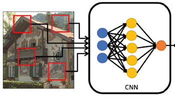
In the testing phase, we follow the typical approach of fusing patch-based predictions as illustrated in Figure 4: to determine an image’s quality, the trained network processes several image patches, yielding one score for each patch. These scores are then averaged to create the final output. When using this patch-based approach, one important design choice is the actual patch size: how much context is needed to predict the overall quality? Research indicates that smaller patches are needed for artificial distortions, while natural distortions require a larger input size [19]. Moreover, good results could only be achieved with sufficient pre-training on large-scale datasets such as ImageNet. This shows that the quality assessment of natural distortions is a more demanding task that needs a larger amount of data. So far, no IQA dataset exists that comes close to a million or more samples, which is not surprising, since label acquisition for IQA is a more intricate task compared to, for example, label acquisition for classification.

The fusing of patch-based predictions relies on the assumption that the scores of the individual patches capture the score of the whole image. This assumption is convenient since one can use several hundred crops per image to train a model, but it is not necessarily valid for all patches. Accordingly, some patches are better suited for prediction. We enhanced our results by selecting patches using an attention model based on the structure tensor.

For artificial distortions, we can assume that small patches already contain sufficient information about perceptual quality. However, the predictive quality of a particular patch heavily depends on the image structure in that patch. The left side of Fig. 3 shows an example of how the predictive quality of patches can vary for jpeg 2000 compression. The right side of Fig. 3 shows the patchwise absolute distance between the ground truth and the local prediction of a CNN. One problem that can be observed is that blurring and compression effects do not alter homogeneous areas, and therefore, no information can be gained there. Hence, one should focus on patches that contain more structure. To this end, we present an effective strategy to sample such patches by using the structure tensor [17]

Ix and Iy are the image derivatives in horizontal- and vertical directions; dΩ is a local region. High values of the determinant of J indicate areas with 2D structure. In our implementation, we first convolved the input image with a Gaussian filter with σpre = 3. We computed the derivatives using Sobel filters. After computing the product terms IxIx, IxIy, and IyIy, we filtered the product terms with a Gaussian filter with σpost = 5 (integration over a local region). We computed the determinant and applied non-maximum suppression in a window of 15 pixels to obtain a feature map, where each pixel encodes the amount of structure (an example is shown in Figure 5). To select the best n patches, we use the top n saliency values and crop patches around the respective center pixel. The pseudo-code for the method is given in Table I. The invariants of the structure tensor have already been used successfully to model human attention and saliency [39], i.e., areas where humans tend to look in an image.

Multiplications of oriented filters, and in general AND operations, can lead to more efficient representation of images [43–45]. Accordingly, we investigated whether AND operations can be helpful in CNN architectures and introduced FP-blocks as additional building blocks for CNNs [11]. Similar to a convolution layer, the input of an FP-block is a 3D tensor with a certain height, width, and depth (number of feature maps). The output is another tensor with possibly a smaller height and width, and usually, an increased depth. A schema of an FP-block is shown in Figure 6 on the right. The input depth din is expanded to q ⋅dout, the desired output depth of the block times an expansion factor q. These new feature maps are created by weighted sums over the input feature maps, an operation implemented by the so-called 1 × 1 convolutions that actually convolve with kernels of size 1 × 1 × din.

Subsequently, the expanded tensor is convolved by two depthwise separable (DWS) convolutions that are then multiplied. In deep-learning jargon, DWS convolutions are convolutions that operate only on one feature map (channel) and not across feature maps. After multiplication, the signal is z-scored (batch normalization without re-scaling) to reduce the risk of vanishing or exploding values. An additional 1 × 1 convolution (weighted summations over feature maps) creates the final output tensor of the FP-block with dout feature maps.

To illustrate how the multiplication of two linear filters can lead to end-stopping, consider an image of a rectangle with horizontal and vertical edges, and two linear filters, one selective to horizontal edges and one to vertical edges. At the corners, both filters would be activated and thus the product would differ from zero. The horizontal edges, however, would only activate the horizontal filter, the vertical edges only the vertical filter, and thus the product would be zero for all straight edges. For a full account on how to model end-stopped neurons based on multiplications of oriented filters see [43].

The essential function of an FP-block is that it multiplies two filtered versions of the same input. In vectorized form, a patch p→, and a filter-pair (fa →,fb →)∈Rk2, k being the kernel size, determine the value g(p→) of the patch’s center pixel as

The output is a weighted sum of k4 possible pixel pairs. In a factorized bilinear layer, as presented by Li et al. [25], the output of each neuron depends on a linear part (not shown here) and a weighted combination of pairwise terms across feature maps. Let x→∈Rn be the vectorization of the d-dimensional input patch P∈Rk x k x d, and n = k2d. The quadratic part of an output neuron is computed by a scalar product of a vector m→0∈Rn2 and the vectorized version of the outer product of x with itself

M∈Rn×n is a reshaped version of m→0 that can be expressed by a factorized matrix V∈Rc×n with vi → being the ith column of V. Arguably, Eq. (7) can be seen as a general case of Eq. (4). However, instead of computing a weighted sum across all feature maps and summing over k4d2 values, we restrict the generation of multiplicative terms to only one feature map at a time. Thus, FP-nets differ from bilinear CNNs in a way similar to how CNNs differ from multilayer perceptrons (MLPs). In addition, the combination of two different filters can result in matrixes W that cannot be reproduced by factorized matrixes M. For example, f→a=(1,0)T and f→b=(0,1)T yield the symmetric 2 × 2 matrix W=12(f→af→bT+f→bf→aT) that has zero entries on the main diagonal and 12 on the top-right and bottom-left positions. No combination of VTV can create such a matrix.

We tested different approaches using FP-nets for three blind IQA datasets. The Legacy dataset contains artificial distortions of high-quality reference images. The LITW and Kon-IQ dataset contain images with natural distortions. For all three benchmarks, the FP-nets were trained on image patches. To infer the overall quality of an image, the values obtained for different patches were averaged. The approaches used for the artificial and authentic datasets differ in the size of a patch, the way patches are selected, the use of pre-training, and the network size. An overview is given in Table III. All experiments were conducted using PyTorch [31].

With LITW, Ghadiyaram and Bovik [10] compiled a demanding benchmark containing 1,162 images with 350,000 scores from over 8,100 human observers. The images were captured mainly by using mobile devices in everyday life situations. Thus, apart from distortions due to the device’s processing chain, image quality can be impaired by the photographer himself, due to over- and underexposure, motion blur, and other sources; see Fig. 1 for examples.

The currently largest labeled dataset with authentic distortions is Kon-IQ [16], containing 10,073 images with 1,2M quality ratings from 1,459 annotators. We trained and evaluated on the small image sizes (512 × 384).

We used the same approach for both datasets: as with the Legacy benchmark, we trained and tested CNNs for 10 different 80/20 splits. On LITW, Kim et al. [19] obtained good results with a pre-trained ResNet-50 and we therefore compared a ResNet-50 with a corresponding FP-net, both pre-trained on ImageNet. We trained both networks for 100 epochs with the Adam optimizer and with learning rate 0.0001 and weight decay 0.001. After the 40th and 80th epoch, the learning rate was reduced by a factor of 0.1. For the 2048-dimensional feature vector right before the linear mapping to the quality score, we used a dropout layer with p = 0.5. Each training mini batch contained 32 patches of size 224 × 224, roughly a quarter of the 500 × 500 dimensional input images. As before, we used the L1-norm as the loss function, vertical flips for data augmentation, and the same normalization as for the Legacy dataset. Due to the large patch size, attention-based patch selection yielded no benefit. Instead of 128 patches, each test image score was predicted with 25 random patches.

To better evaluate the generalization capabilities of the models, all networks trained on LITW were tested on the full Kon-IQ dataset and vice versa.

In addition to the performance scores, we report the number of parameters in millions (M) to compare for efficiency. If possible, we determined the number of parameters from the respective paper’s description. In many cases, the CNNs used in the literature are large and were combined with even larger MLPs. In those cases, we report only the CNN’s standard size as a lower bound. A “ >” denotes that the size is even larger due to, for example, an additional MLP. Note that with the FP-nets, no additional regression models were used. We do not report the number of parameters for BRISQUE [29] and CORNIA [42].

Figure 10 presents results for all configurations tested on the Legacy dataset. First, note that our simple attention model (denoted by J) increased the median PLCC by 0.2% for the ResNet, and by 0.4% for the FP-nets I and II (with % we denote an absolute increase of 1/100, for example, 0.975 with an 0.2% increase yields 0.977). Also, note that the FP-nets with attention model outperformed the ResNet by 0.2%. As shown in Table IV, the fact that FP-nets yield results comparable to the state of the art is remarkable since the number of parameters is reduced by a substantial amount. Furthermore, we were able to outperform the FP-net I in terms of mean PLCC by 0.1% using the FP-net II architecture (the minimum and maximum PLCC values also increased) with even fewer convolution layers and parameters. Note that the SROCC scores of both FP-nets are better than the ResNet-32’s and that the attention mechanism increased the SROCC scores of all three architectures. The results for the ten splits of the LITW dataset are shown in Figure 11. Here, the FP-net has a higher variance (0.021 versus 0.015) with a lower minimum and a higher maximum score. The mean value is decreased by 0.3% (0.859 versus 0.856), the median value is decreased by 0.2% (0.860 versus 0.858). Nevertheless, these results show that a comparable performance is possible with fewer convolution layers and significantly fewer parameters. Table V shows results for further state-of-the-art approaches on the LITW dataset.

Regarding the Kon-IQ results shown in Table VI, the FP-net performed on par with the ResNet-50 baseline. A similar outcome can be observed for the cross-database results in Table VII. Here, the differences between the mean PLCC and SROCC values are within one standard deviation (that was equal for the ResNet-50 and the FP-net). When trained on LITW and evaluated on Kon-IQ, the standard deviation was 0.01. When trained on Kon-IQ and evaluated on LITW, the standard deviations were 0.005 and 0.004 for PLCC and SROCC, respectively.

We used FP-nets to model perceptual image quality and obtained state-of-the-art results with fewer parameters and fewer layers. This increased efficiency was obtained by substituting generic convolutional blocks with the so-called FP-blocks that employ multiplications of feature maps.

FP-blocks are inspired by characteristics of end-stopped cells in biological visual systems; these cells can be modeled by multiplications of orientation-selective filters and provide efficient 2D representations. Since image quality assessment is based on human perception, models based on principles of human vision should be beneficial. The effectiveness of multiplicative terms and salient 2D representations is further illustrated by the attention model that we use for patch sampling.

An additional explanation of why FP-nets work well may be that they provide a second-order polynomial kernel that increases the layer’s capacity and therefore reduces the number of layers needed.

We conclude that inspiration from research on human vision can still provide useful ideas for the design of deep networks beyond just convolutions and pooling. The FP-nets in particular seem well-suited for predicting subjective image quality with rather compact network models.

References

1BarthE.WatsonA. B.2000A geometric framework for nonlinear visual codingOpt. Express7155165155–6510.1364/OE.7.000155
2BerkesP.WiskottL.2006On the analysis and interpretation of inhomogeneous quadratic forms as receptive fieldsNeural Comput.18186818951868–9510.1162/neco.2006.18.8.1868
3BergstraJ.DesjardinsG.LamblinP.BengioY.2009Quadratic polynomials learn better image featuresTech. report1337
4BiancoS.CelonaL.NapoletanoP.SchettiniR.2018On the use of deep learning for blind image quality assessmentSignal, Image Video Process.12355362355–6210.1007/s11760-017-1166-8
5BosseS.ManiryD.WiegandT.SamekW.A deep neural network for image quality assessment2016 IEEE Int’l. Conf. on Image Processing (ICIP)2016IEEEPiscataway, NJ377337773773–7
6ChengZ.TakeuchiM.KattoJ.A pre-saliency map based blind image quality assessment via convolutional neural networks2017 IEEE Int’l. Symposium on Multimedia (ISM)2017IEEEPiscataway, NJ778277–82
7ChowdhuryA. R.LinT.-Y.MajiS.Learned-MillerE.One-to-many face recognition with bilinear cnns2016 IEEE Winter Conf. on Applications of Computer Vision (WACV)2016IEEEPiscataway, NJ191–9
8DengJ.DongW.SocherR.LiL.-J.LiK.Fei-FeiL.ImageNet: A large-scale hierarchical image database2009 IEEE Conf. Comput. Vis. Pattern Recognit.2009IEEEPiscataway, NJ248255248–55
9GaoY.BeijbomO.ZhangN.DarrellT.Compact bilinear poolingProc. IEEE Conf. on Computer Vision and Pattern Recognition2016IEEEPiscataway, NJ317326317–26
10GhadiyaramD.BovikA. C.2015Massive online crowdsourced study of subjective and objective picture qualityIEEE Trans. Image Process.25372387372–8710.1109/TIP.2015.2500021
11GrüningP.MartinetzT.BarthE.“Feature products yield efficient networks,” Preprint arXiv:2008.07930 (2020)
12HanD.KimJ.KimJ.Deep pyramidal residual networksProc. IEEE Conf. on Computer Vision and Pattern Recognition2017IEEEPiscataway, NJ592759355927–35
13HeK.ZhangX.RenS.SunJ.Deep residual learning for image recognitionProc. IEEE Conf. on Computer Vision and Pattern Recognition2016IEEEPiscataway, NJ770778770–8
14HuJ.ShenL.SunG.Squeeze-and-excitation networksProc. IEEE Conf. on Computer Vision and Pattern Recognition2018IEEEPiscataway, NJ713271417132–41
15HubelD. H.WieselT. N.1965Receptive fields and functional architecture in two nonstriate visual areas (18 and 19) of the catJ. Neurophysiol.28229289229–8910.1152/jn.1965.28.2.229
16HosuV.LinH.SziranyiT.SaupeD.2020KonIQ-10k: An ecologically valid database for deep learning of blind image quality assessmentIEEE Trans. Image Process.29404140564041–5610.1109/TIP.2020.2967829
17JähneB.Spatio-Temporal Image Processing: Theory and Scientific Applications1993Vol. 751SpringerBerlin
18KangL.YeP.LiY.DoermannD.Convolutional neural networks for no-reference image quality assessmentProc. IEEE Conf. on Computer Vision and Pattern Recognition2014IEEEPiscataway, NJ173317401733–40
19KimJ.ZengH.GhadiyaramD.LeeS.ZhangL.BovikA. C.2017Deep convolutional neural models for picture quality predictionIEEE Signal Process. Mag.34130141130–4110.1109/MSP.2017.2736018
20KimJ.NguyenA.-D.LeeS.2018Deep CNN-based blind image quality predictorIEEE Trans. Neural Netw. Learn. Syst.30112411–2410.1109/TNNLS.2018.2829819
21KrizhevskyA.SutskeverI.HintonG. E.2012Imagenet classification with deep convolutional neural networksAdv. Neural Inf. Process. Syst.25109711051097–105
22KrizhevskyA.NairV.HintonG.“CIFAR-10 (Canadian Institute for Advanced Research),” (2020)
23LarsonE. C.ChandlerD. M.2010Most apparent distortion: full-reference image quality assessment and the role of strategyJ. Electron. Imaging191100610.1117/1.3267105
24LinT.-Y.RoyChowdhuryA.MajiS.Bilinear CNN models for fine-grained visual recognitionProc. IEEE Int’l. Conf. on Computer Vision2015IEEEPiscataway, NJ144914571449–57
25LiY.WangN.LiuJ.HouX.Factorized bilinear models for image recognitionProc. IEEE Int’l. Conf. on Computer Vision2017IEEEPiscataway, NJ207920872079–87
26LiX.WangW.HuX.YangJ.Selective kernel networksProc. IEEE Conf. on Computer Vision and Pattern Recognition2019IEEEPiscataway, NJ510519510–9
27LiuX.van de WeijerJ.BagdanovA. D.Rankiqa: Learning from rankings for no-reference image quality assessmentProc. IEEE Int’l. Conf. on Computer Vision2017IEEEPiscataway, NJ104010491040–9
28MaK.LiuW.ZhangK.DuanmuZ.WangZ.ZuoW.2018End-To-end blind image quality assessment using deep neural networksIEEE Trans. Image Process.27120212131202–1310.1109/TIP.2017.2774045
29MittalA.MoorthyA. K.BovikA. C.2012No-reference image quality assessment in the spatial domainIEEE Trans. image Process.21469547084695–70810.1109/TIP.2012.2214050
30MotaC.BarthE.2000On the uniqueness of curvature featuresDynamische Perzeption9175178175–8
31PaszkeA.GrossS.MassaF.LererA.BradburyJ.ChananG.KilleenT.LinZ.GimelsheinN.AntigaL.DesmaisonA.KöpfA.YangE.DeVitoZ.RaisonM.TejaniA.ChilamkurthyS.SteinerB.FangL.BaiJ.ChintalaS.WallachH.LarochelleH.BeygelzimerA.d’Alché-BucF.FoxE.GarnettR.PyTorch: An Imperative style, high-performance deep learning libraryAdvances in Neural Information Processing Systems 322019Curran AssociatesRed Hook, NY, USA802480358024–35
32PonomarenkoN.JinL.IeremeievO.LukinV.EgiazarianK.AstolaJ.VozelB.ChehdiK.CarliM.BattistiF.KuoC.-C. J.2015Image database TID2013: Peculiarities, results and perspectivesSignal Process. Image Commun.30577757–7710.1016/j.image.2014.10.009
33PeiS. C.ChenL. H.2015Image quality assessment using human visual DOG model fused with random forestIEEE Trans. Image Process.24328232923282–9210.1109/TIP.2015.2440172
34SimonyanK.ZissermanA.“Very deep convolutional networks for large-scale image recognition,” CoRR, vol. abs/1409.1 (2014) arXiv preprint arXiv:1409.1556 pp. 1–14
35SheikhH. R.SabirM. F.BovikA. C.2006A statistical evaluation of recent full reference image quality assessment algorithmsIEEE Trans. image Process.15344034513440–5110.1109/TIP.2006.881959
36TuZ.WangY.BirkbeckN.AdsumilliB.BovikA. C.“UGC-VQA: Benchmarking blind video quality assessment for user generated content,” arXiv, pp. 1–13, (2020)
37UstinovaE.GaninY.LempitskyV.Multi-region bilinear convolutional neural networks for person re-identification2017 14th IEEE Int’l. Conf. on Advanced Video and Signal Based Surveillance (AVSS)2017IEEEPiscataway, NJ161–6
38VargaD.SaupeD.SzirányiT.DeepRN: A content preserving deep architecture for blind image quality assessment2018 IEEE Int’l. Conf. on Multimedia and Expo (ICME)2018IEEEPiscataway, NJ161–6
39VigE.DorrM.MartinetzT.BarthE.2012Intrinsic dimensionality predicts the saliency of natural dynamic scenesIEEE Trans. Pattern Anal. Mach. Intell.34108010911080–9110.1109/TPAMI.2011.198
40VolterraV.Theory of Functionals and of Integral and Integro-differential Equations1959Dover, New York
41WangQ.WuB.ZhuP.LiP.ZuoW.HuQ.“ECA-net: Efficient channel attention for deep convolutional neural networks,” Preprint arXiv:1910.03151 (2019)
42YeP.KumarJ.KangL.DoermannD.Unsupervised feature learning framework for no-reference image quality assessment2012 IEEE Conf. on Computer Vision and Pattern Recognition2012IEEEPiscataway, NJ109811051098–105
43ZetzscheC.BarthE.1990Fundamental limits of linear filters in the visual processing of two-dimensional signalsVis. Res.30111111171111–710.1016/0042-6989(90)90120-A
44ZetzscheC.BarthE.Image surface predicates and the neural encoding of two-dimensional signal variationHuman Vision and Electronic Imaging: Models, Methods, and Applications1990Vol. 1249SPIEBellingham, WA160177160–77
45ZetzscheC.BarthE.WegmannB.WatsonA. B.The importance of intrinsically two-dimensional image features in biological vision and picture codingDigital Images and Human Vision1993MIT PressCambridge109138109–38
46ZhaiG.MinX.2020Perceptual image quality assessment: a surveySci. CHINA Inf. Sci.6321130110.1007/s11432-019-2757-1
47ZhangW.MaK.YanJ.DengD.WangZ.“Blind image quality assessment using a deep bilinear convolutional neural network”, IEEE Trans. Circuits Syst. Video Technol. 30, 36–47 (2018)
48ZhouB.LapedrizaA.KhoslaA.OlivaA.TorralbaA.2017Places: A 10 million image database for scene recognitionIEEE Trans. Pattern Anal. Mach. Intell.40145214641452–6410.1109/TPAMI.2017.2723009
49ZoumpourlisG.DoumanoglouA.VretosN.DarasP.Non-linear convolution filters for CNN-based learningProc. IEEE Int’l. Conf. on Computer Vision2017IEEEPiscataway, NJ476147694761–9