Analyzing the Impact of Color Spaces and Color Augmentation on Material Segmentation and Feature&#xA0;Representation

Soroush Shahbaznejad; Mekides Assefa Abebe; Alireza Rabbanifar; Michael J. Murdoch

doi:10.2352/J.ImagingSci.Technol.2026.70.5.050402

Abstract

Material segmentation hinges on pixel-level cues in hue, chroma, and lightness, yet most pipelines remain in device-referred sRGB and use ad hoc photometric tweaks. The authors disentangle the effects of color encoding versus principled, opponent-axis augmentations by training the same FCN–ResNet101 across a 3 × 4 grid: three encodings (sRGB, CIELAB, YCbCr) and three colorimetric perturbations—luminance translation (brightness), luminance scaling (contrast), and chroma-magnitude scaling (saturation)—plus a no-augmentation baseline. Using overlap-aware metrics (intersection over union; F₁) and confirmatory mixed-effects analyses, they find that augmentation—not encoding—is the primary driver of accuracy. Contrast (luminance scaling) delivers the most reliable global gains; brightness is especially effective for specular materials (metal, glass) while saturation benefits chroma-dominant diffuse classes (paper, fruits). Color encoding acts as a secondary modulator: YCbCr’s luminance–chrominance separation sharpens neutral or composite boundaries (e.g., plastic), whereas CIELAB’s approximate perceptual uniformity aids materials with broader chroma spread. Qualitative overlays and backbone-feature embeddings via t-distributed stochastic neighbor embedding (t-SNE) corroborate these trends, showing cleaner boundaries and more separable latent clusters under luminance-scaled training. Practically, the authors recommend contrast as the safe default, favoring YCbCr when specular cues dominate and CIELAB when chroma carries the signal.

jist

JIMTE6

Journal of Imaging Science and Technology

J. Imaging Sci. Technol.

1062-3701

1943-3522

Society for Imaging Science and Technology

050402

10.2352/J.ImagingSci.Technol.2026.70.5.050402

2025011

Work Presented at Electronic Imaging 2026

Analyzing the Impact of Color Spaces and Color Augmentation on Material Segmentation and Feature Representation

Analyzing the impact of color spaces and color augmentation on material segmentation and feature representation

ShahbaznejadSoroush

AbebeMekides Assefa

RabbanifarAlireza

MurdochMichael J.

Munsell Color Science Laboratory, Rochester Institute of Technology, Rochester, NY 14623, USA

ss3105@g.rit.edu

Shahbaznejad et al.

092026

982025

452026

2026

Abstract

Material segmentation hinges on pixel-level cues in hue, chroma, and lightness, yet most pipelines remain in device-referred sRGB and use ad hoc photometric tweaks. The authors disentangle the effects of color encoding versus principled, opponent-axis augmentations by training the same FCN–ResNet101 across a 3 × 4 grid: three encodings (sRGB, CIELAB, YCbCr) and three colorimetric perturbations—luminance translation (brightness), luminance scaling (contrast), and chroma-magnitude scaling (saturation)—plus a no-augmentation baseline. Using overlap-aware metrics (intersection over union; F1) and confirmatory mixed-effects analyses, they find that augmentation—not encoding—is the primary driver of accuracy. Contrast (luminance scaling) delivers the most reliable global gains; brightness is especially effective for specular materials (metal, glass) while saturation benefits chroma-dominant diffuse classes (paper, fruits). Color encoding acts as a secondary modulator: YCbCr’s luminance–chrominance separation sharpens neutral or composite boundaries (e.g., plastic), whereas CIELAB’s approximate perceptual uniformity aids materials with broader chroma spread. Qualitative overlays and backbone-feature embeddings via t-distributed stochastic neighbor embedding (t-SNE) corroborate these trends, showing cleaner boundaries and more separable latent clusters under luminance-scaled training. Practically, the authors recommend contrast as the safe default, favoring YCbCr when specular cues dominate and CIELAB when chroma carries the signal.

material segmentationsemantic segmentationdeep learningcolor spaces (CIELABYCbCrsRGB)color-based augmentation

ccc

1062-3701/2026/70(5)/050402/15/$25.00

printed

Printed in the USA

Introduction

1.1

Motivation and Prior Work

Material segmentation assigns a material label—metal, glass, fabric, and so on—to every pixel in an image. Reliable pixel-level maps unlock a spectrum of downstream technologies across diverse applications. For example, in robotics, grasp planners must modulate contact force and approach angles according to surface compliance, necessitating that manipulators accurately distinguish smooth plastic from rough ceramic before physical contact [1]. Similarly, photorealistic augmented-reality pipelines require detailed bidirectional reflectance distribution functions for each surface to ensure virtual shadows and highlights seamlessly align with real-world materials [2]. In autonomous driving, distinguishing high-gloss traffic signs from diffuse asphalt is essential for reliable scene interpretation. Industrial inspection workflows, meanwhile, depend heavily on identifying incomplete welds or varnish defects that lack clear geometric or shape-based cues [3, 4]. Central to accurate material perception—by humans or machines—are color cues: hue, chroma, and lightness. These attributes provide powerful indicators: oxidized steel typically resides in low-chroma, high-lightness regions of color space while ripe fruits cluster around highly saturated reds and yellows. Despite the established significance of perceptual color spaces, most convolutional neural networks (CNNs) continue to rely on device-dependent sRGB values. However, the sRGB transfer function was designed for legacy CRT displays, and its axes neither maintain perceptual uniformity nor decorrelate chromatic attributes from luminance. In contrast, CIELAB approximately linearizes perceptual distances and YCbCr separates luminance (luma) from chromatic components. Although color science consistently advocates perceptually coherent spaces for reliable distance metrics, rigorous end-to-end evaluations within modern CNNs remain sparse [5].

Data augmentation is essential for modern segmentation accuracy because it synthetically enlarges the training set, reduces overfitting, and improves generalization [6]. In practice, pipelines emphasize geometric transformations (random cropping, horizontal flipping, rotation, scaling, perspective warping), which encourage invariance to viewpoint and object location and thereby improve accuracy across diverse real-world camera perspectives [7]. Color augmentations are used less systematically: typical routines apply global brightness/contrast/saturation/hue adjustments in sRGB, and policy-search methods like AutoAugment and RandAugment likewise focus on sRGB [8]. Strong color perturbations (large hue shifts or aggressive brightness/saturation) can degrade performance by pushing samples far from the training distribution [8, 9]. Conversely, Abebe et al. showed in skin segmentation that strong brightness augmentation can substantially improve robustness to exposure variation, whereas equivalently strong saturation changes provide limited benefit [10]. These mixed outcomes raise a natural question: Does the color-space choice—sRGB versus perceptually informed encodings like CIELAB or luminance–chroma–decorrelated YCbCr—govern how helpful a given color augmentation is for material segmentation?

1.1.1

Psychophysics and Color/Appearance Priors

A large body of psychophysics demonstrates that the perceived material category depends jointly on chromaticity, lightness, gloss, and translucency cues. Fleming’s review synthesizes how highlights and shading statistics signal specularity and translucency across materials [3]. Subsequent studies show that color, gloss, and translucency behave as statistically independent perceptual dimensions, supporting the idea of manipulating luminance and chroma along opponent axes without collapsing categories [11]. Related work on gloss constancy and illumination variation further highlights the role of lightness gradients and specular structure in material judgments [12]. These findings motivate augmentations that (i) treat luminance separately from chroma and (ii) preserve hue while scaling chroma magnitude—precisely the operations that are natural in CIELAB (L, a, b) and YCbCr (Y, Cb, Cr) but not in gamma-encoded sRGB.

1.1.2

Color Spaces, Robustness, and What CNNs Actually Learn

Engineering studies corroborate these perceptual priors: for pixelwise inspection and outdoor scene understanding, CIELAB and YCbCr often outperform sRGB when decisions hinge on chroma–luminance structure rather than raw device triplets [13, 14]. At the representation level, ImageNet-trained CNNs are known to be texture-biased, with early layers learning color-opponent filters but deeper layers entangling texture and color [15]. This texture bias can obscure material boundaries when color statistics shift. Robustness work and augmentation surveys emphasize that luminance-centric edits (contrast/brightness) tend to improve downstream performance and stability more reliably than arbitrary hue jitter, especially when applied in opponent spaces that avoid hue drift [6, 9]. In semantic segmentation specifically, De and Pedersen reported that strong chromatic shifts can sharply degrade accuracy on ADE20K, underscoring the need for principled, space-aware color perturbations [16]. Together, these results suggest that color augmentation should be expressed in perceptually structured spaces if we require invariance to illumination without corrupting diagnostic hue/chroma cues.

1.1.3

Research Gap and Proposed Approach

Despite this converging evidence, most end-to-end segmentation pipelines still (i) train in sRGB, (ii) apply color jitter in the same space, and (iii) do not disentangle augmentation strength from the choice of pixel encoding. Accordingly, we systematically evaluate brightness, contrast, and saturation applied in sRGB, CIELAB, and YCbCr within a fixed fully convolutional network (FCN)–ResNet101, isolating augmentation from encoding in a 3 × 4 design and analyzing both accuracy and learned color representations.

1.2

Problem Statement and Contributions

1.2.1

Research Question

How do brightness, contrast, and saturation augmentations—applied independently in sRGB, CIELAB, and YCbCr—affect the accuracy of a CNN-based material-segmentation model, and how do they reshape its internal color representations? We specifically examine how each augmentation–color-space pairing redistributes material clusters in (i) pixel-level color spaces and (ii) high-dimensional learned embeddings, with implications for robustness in photometrically demanding scenarios.

1.2.2

Objectives and Contributions

To answer this question, we pursue three objectives without altering network architecture or training protocol:

(1)

Quantify augmentation effects across color spaces. We measure how brightness, contrast, and saturation individually influence segmentation accuracy when applied in sRGB, CIELAB, and YCbCr. To our knowledge, this is the first comprehensive comparison of these augmentations across multiple perceptually meaningful encodings within a fixed FCN–ResNet101 backbone.

(2)

Compare effects across diverse materials. UsingCOCO–Materials—a mapping of 27 COCO object classes to eight material categories (55,492 training and 2385 validation images)—we quantify augmentation effects systematically across materials, providing benchmarks and guidelines tailored to material segmentation.

(3)

Analyze and interpret learned color embeddings. Using t-distributed stochastic neighbor embedding (t-SNE), we visualize how augmentations reshape learned feature representations. We provide a color-appearance-informed interpretation and extend brightness-robustness insights from [10] to a broader range of materials.

This integrated treatment links color appearance to deep feature learning and supports scientifically grounded augmentation strategies for vision tasks where color is a first-order cue.

Methodology

This section describes the pipeline used to systematically investigate how color-centric data augmentation and the choice of color space influence material-segmentation accuracy and reshape the internal feature representations learned by CNNs.

As shown in Figure 1, the methodology consists of preparing a COCO-based material dataset, selecting a representative semantic-segmentation model, and applying color augmentations in multiple color spaces. The model is trained with and without these augmentations, and the results are analyzed per material and via representation diagnostics.

Figure 1.

Top: End-to-end pipeline for material segmentation, from COCO image + polygons through material mapping, mask rasterization, color-space conversion (sRGB/YCbCr/CIELAB), single-attribute color augmentation (ΔB, ΔC, ΔS), to prediction and metric computation (BCE, IoU, F1). Bottom: FCN–ResNet101 backbone with a 1 × 1 auxiliary head and 3 × 2 bilinear upsampling for dense material logits, improving gradient flow [17].

2.1

Dataset Preparation

2.1.1

COCO-2017 Base and Material Mapping

The COCO dataset [18] provides polygonal instance masks for 80 object categories across the train (118k images), val (5k), and test (41k) splits. We use the train and val splits (about 123k images total) with per-instance masks. From COCO’s 80 classes, we identified 27 whose typical appearance is dominated by one of eight material types (e.g., metal, plastic, glass). Two color-science experts independently assigned the 27 object categories to the eight material bins and resolved disagreements by majority vote, yielding the COCO–Materials mapping (Table I) with 55,492 training and 2,385 validation images.

Table I.

Material categories, mapped COCO classes, and instance counts.

Material	COCO classes	Rrain	Val
Metal	Fork, Spoon, Knife	11,410	489
Plastic	Keyboard, Remote, Frisbee, Sports Ball	11,637	504
Glass	Wine Glass, Vase, TV	10,687	454
Fruits	Banana, Apple, Orange, Broccoli, Carrot	9,150	416
Feather	Bird	3,237	125
Animal hair	Horse, Dog, Cat, Sheep, Cow, Bear, Zebra, Giraffe	20,359	876
Paper	Book	5,332	230
Ceramic	Bowl, Toilet	10,464	463

Figure 2 shows three examples: (a) the original COCO image, (b) instance-level COCO masks for the selected object classes, and (c) the aggregated material masks resulting from the class-to-material mapping.

Figure 2.

Material mapping examples. Each row shows (a) the original COCO image, (b) instance masks with COCO object labels, and (c) the corresponding material masks, illustrating: animal hair + ceramic, metal + fruit, and glass + plastic.

2.1.2

Rasterization and Dataset Splitting

The COCO instances are annotated as polygons. We rasterized polygons to per-pixel masks using pycocotools and manually verified 500 randomly sampled polygons for fidelity. We then filtered the train/val splits to retain images containing at least one of the 27 selected object classes, yielding 55,492 training and 2385 validation images (summing the per-material counts in Table I). To standardize inputs for FCN–ResNet101, each image was center-cropped and bilinearly resized to 512 × 512 pixels; the same transform was applied to the multi-material masks. These pairs constitute the dataset used in all experiments.

2.1.3

Color Distributions Across Material Classes

We visualize per-pixel color statistics in Figure 3: (a) sRGB chromaticity (red versus green), (b) CIELAB a∗b∗ (opponent-chroma axes), and (c) YCbCr CbCr (decorrelated chroma components). Solid ellipses denote the 95% covariance regions for each material, revealing intrinsic chromatic variance and overlap.

Figure 3.

Per-pixel color distributions for the eight material categories: (a) sRGB chromaticity, (b) CIELAB a∗b∗, and (c) YCbCr CbCr. Ellipses mark 95% covariance regions.

2.1.4

Interpretation

The key observations from Fig. 3 are as follows: (i) wide chromatic spreads for fruits (e.g., broccoli, carrot, apple) and metal (specular highlights, color casts); (ii) compact clusters for animal hair and paper despite large sample counts; (iii) moderate variance for plastic—many neutral items with occasional strong hues (e.g., Frisbees); (iv) CIELAB/YCbCr often separate materials more clearly than sRGB, consistent with perceptual uniformity or luma–chroma decorrelation. These patterns track each material’s inherent color diversity more than raw image counts, suggesting that robustness hinges on color spaces and augmentations aligned with natural appearance.

2.2

Image Augmentation

We isolate the effect of color augmentations (Albumentations [19]) on material segmentation [6]. Following policy-learning work [8], we vary brightness, contrast, and saturation in three pixel encodings (sRGB, YCbCr, CIELAB). To ensure reproducibility, we specify the exact conversions, units, parameter grids, and clipping rules.

2.2.1

Color-Space Conventions and Conversions

sRGB (IEC 61966-2-1) [20]: Images are read/written as gamma-encoded sRGB. Unless noted, augmentations in the “sRGB” condition operate in this nonlinear domain (as in Albumentations [19]). When HSV is used, we convert sRGB → HSV on [0, 1] floats and back.

YCbCr (BT.601, full range/JPEG style) [21–23]: We use full-range YCbCr (not studio limited). For R, G, B ∈ [0,255],

\begin{matrix} Y = 0.299 R + 0.587 G + 0.114 B, \\ C_{b} = 128 - 0.168736 R - 0.331264 G + 0.5 B, \\ C_{r} = 128 + 0.5 R - 0.418688 G - 0.081312 B, \end{matrix}

so Y ∈ [0,255] and Cb, Cr ∈ [0,255] (128 is neutral). This is implemented with OpenCV’s full-range conversion (float32 internally; clip to [0, 255] on write).

CIELAB (D65 reference white) [24, 25]: sRGB → linear RGB (inverse EOTF) → XYZ(D65) → CIELAB using D65 white (no chromatic adaptation). Thus L∗∈ [0,100], a∗, b∗≈ [− 110,110]. When required, we use L∗Cab∗h∗ with

C_{a b}^{*} = \sqrt{a^{* 2} + b^{* 2}}

All augmentations follow convert→augment in native space→convert back to sRGB (float32). Componentwise clipping is applied in the working space before conversion back to sRGB, and the final sRGB is clipped to [0, 1] (or [0, 255] for 8-bit exports).

2.2.2

Parameterization (Shared Across Spaces)

We use the same dimensionless step sizes in each space by normalizing the luminance/lightness channel to [0, 1] and expressing saturation as a multiplicative chroma scale. The five levels for training/test sweeps are

Δ B, Δ C, Δ S \in {- 0.30, - 0.10, 0, 0.10, 0.30} .

These form the weak → strong ladder shown in Figure 4.

Figure 4.

Representative strength ladder for the three color augmentations (brightness, contrast, saturation) applied in sRGB, CIELAB, and YCbCr. Each training (and test) image is augmented at six levels, indicated on the left of each row.

2.2.3

Exact Per-Space Transforms

Brightness (operate on Y or L∗, unified by normalization):

\begin{matrix} \tilde{L} = \frac{L}{L_{max}}, \\ {\tilde{L}}^{'} = clip (\tilde{L} + Δ B, 0, 1), \\ L^{'} = {\tilde{L}}^{'} L_{max}, \end{matrix}

where (L, Lmax) = (L∗, 100) in CIELAB and (L, Lmax) = (Y, 255) in YCbCr. In the sRGB condition, we operate on HSV value V ∈ [0,1] as V ′ = clip(V + ΔB, 0,1)(note that HSV V is not photometric luminance; we retain this for consistency with common libraries).

Contrast (scale deviations about the channel mean

\bar{L}

\begin{matrix} \tilde{L} = \frac{L}{L_{max}}, \bar{\tilde{L}} = mean (\tilde{L}), \\ {\tilde{L}}^{'} = clip ((\tilde{L} - \bar{\tilde{L}}) (1 + Δ C) + \bar{\tilde{L}}, 0, 1), \\ L^{'} = {\tilde{L}}^{'} L_{max} . \end{matrix}

Same channels as brightness: L∗ (CIELAB), Y (YCbCr), or V (HSV in sRGB).

Saturation/chroma (scale chroma magnitude; preserve hue):

CIELAB: convert to L∗C∗h∗. Define and with

C_{a b}^{*} = \sqrt{a^{* 2} + b^{* 2}}

\begin{matrix} C_{a b}^{*'} = clip ((1 + Δ S) C_{a b}^{*}, 0, C_{max}^{*}), \\ γ = \{\begin{matrix} C_{a b}^{*'} ∕ C_{a b}^{*}, & C_{a b}^{*} > 0, \\ 1, & C_{a b}^{*} = 0, \end{matrix} \\ a^{*'} = γ a^{*}, b^{*'} = γ b^{*} . \end{matrix}

Gamut is enforced by CIELAB→sRGB conversion and final sRGB clipping.

∙

YCbCr: zero-center chroma and scale

\begin{matrix} C_{b}^{'} = 128 + (1 + Δ S) (C_{b} - 128), \\ C_{r}^{'} = 128 + (1 + Δ S) (C_{r} - 128), \end{matrix}

and then clip Cb′, Cr′∈ [0,255].

∙

sRGB: convert to HSV, scale S as

S^{'} = clip ((1 + Δ S) S, 0, 1),

preserve H, and then convert back to sRGB.

2.2.4

Implementation Notes

All operations are performed in float32; conversions follow the references cited previously. We do not linearize sRGB for these jitter operations (matching Albumentations defaults [19]); luminance/lightness manipulations are performed in Y, L∗, or V as specified. “No-Aug” models undergo color-space conversion (for YCbCr/CIELAB training) without attribute perturbation. The CIELAB-chroma scaling may induce out-of-gamut colors; we accept mild clipping on return to sRGB rather than pre-warping the gamut [25, 26].

2.2.5

Protocol

Each training image receives exactly one augmentation at one of five nonzero strengths or identity, yielding six variants per color space. Figure 4 shows representative strengths; this exposes the model to a broad photometric spectrum and encourages learning material-intrinsic cues.

2.3

Model and Training

To evaluate the color-space × augmentation design described above, we train FCN–ResNet101 across 12 combinations: three color spaces (sRGB, CIELAB, YCbCr) and four augmentation policies (None, Brightness, Contrast, Saturation). For each combination, we select the checkpoint with the lowest validation loss. Figure 1 summarizes the pipeline and model.

2.3.1

FCN–ResNet101 Architecture

We adopt the FCN with a ResNet101 backbone as in [17], chosen for strong performance and simplicity. The ResNet101 encoder produces the deepest feature map (2048 channels) that is projected to 27 logits via a 1 × 1 convolution and then upsampled 32× by bilinear interpolation to input resolution. An auxiliary head at stride 16 also predicts 27-channel logits trained with a binary cross-entropy (BCE) loss identical to the main head. This lean decoder minimizes confounds, so differences arise from color/augmentation choices (Section 1.2).

2.3.2

Training Protocol

All runs share identical optimization: RMSProp [27] with learning rate 5 × 10−5, momentum 0.9, weight decay 10−5, and batch size 16 (eight images/two NVIDIA A40 GPUs). We reduce the learning rate by 0.1 after four plateau epochs and train up to 75 epochs with early stopping (no validation-loss improvement for 15 epochs) [28]. The final evaluation uses the checkpoint with the lowest validation BCE; we report per-material intersection over union (IoU), F1, Precision, and Recall on the held-out test split.

2.3.3

Evaluation and Feature Representation Analysis

We report standard pixel-level metrics and overlap-aware losses, citing the original (or canonical) sources for each definition. For each material, we compute the following:

Precision [29]

Precision = \frac{T P}{T P + F P} .

Recall [29]

Recall = \frac{T P}{T P + F N} .

F1/Dice [30]

F_{1} = Dice = \frac{2 T P}{2 T P + F P + F N} .

IoU [31]

IoU = \frac{T P}{T P + F P + F N} .

Soft-IoU loss (Jaccard with soft labels) [32]

L_{IoU} = 1 - \frac{\sum_{i} p_{i} t_{i}}{\sum_{i} p_{i} + \sum_{i} t_{i} - \sum_{i} p_{i} t_{i}} .

Tversky loss [33]

L_{T} = 1 - \frac{T P}{T P + α F P + β F N}, (α, β) = (0.3, 0.7) .

For visualization, we negate loss values so that “higher is better” while statistical analyses use the raw (positive) losses. For representation analysis, we extract stride-16 feature maps, average-pool to 512-D per image, and embed via t-SNE; cluster separability under each color-space × augmentation condition (Figure 11) links metric gains to changes in learned color semantics.

2.3.4

Experimental Design and Representation Analysis

Following a 3 × 4 × 3 factorial design (color space × augmentation × seed), we train 36 models and evaluate each on the same 81-image test split. Beyond aggregate metrics, we visualize the 512-D pooled features using t-SNE to assess how material clusters separate under different color treatments (Fig. 11), directly addressing Objective (3).

Results

3.1

Training Dynamics

Figure 5 plots the mean BCE over epochs for all 3 × 4 color-space × augmentation conditions (Section 2.3). The top row shows training loss and the bottom row validation loss; the left column isolates Brightness to make color-space effects visible, and the right column overlays all runs. Loss drops sharply in the first ∼5 epochs (to BCE ≈ 0.045) and then plateaus. Validation loss bottoms out around epochs 3–4 (≈0.007) and rises mildly thereafter, so the early-stopping protocol in Section 2.3 avoids overfitting. Importantly, curves are nearly superposed across conditions: BCE, which penalizes per-pixel probability miscalibration, becomes insensitive once coarse structure is learned. Subsequent analyses therefore rely on the overlap-centric metrics from Section 2.3 (IoU, F1, Soft-IoU, Tversky) that are sensitive to boundary quality and class imbalance.

Figure 5.

Training and validation BCE. Mean BCE across the 3 × 4 color-space–augmentation grid (Section 2.3). Rows: training (top) and validation (bottom); left: Brightness only; right: all runs overlaid. Curves converge quickly and are nearly indistinguishable across conditions, motivating overlap-centric metrics (Section 2.3).

3.1.1

Why BCE Conceals Differences

The BCE treats pixels independently and saturates once global structure is captured. The IoU and Tversky weight region overlap and asymmetry (Section 2.3); these highlight boundary refinements and minority-class behavior that depend on color space and augmentation.

3.2

Global Accuracy Patterns

Before inferential testing, we first summarize empirical distributions of the evaluation metrics on the 81-image test split (Section 2.3). Figure 6 shows violin plots (with all observations and quartiles) for Precision, Recall, IoU, and F1 within each color space. Medians for Precision, IoU, and F1 are nearly coincident across sRGB, CIELAB, and YCbCr, and their interquartile ranges largely overlap. Recall exhibits the broadest spread—consistent with the material-level variability detailed later—yet the central tendency remains similar across spaces. In short, simply re-encoding images (without augmentation) does not materially change aggregate accuracy.

Figure 6.

Metric distributions by color space (test n = 81). Violin plots with all samples overlaid show that sRGB, CIELAB, and YCbCr have very similar medians and spreads for Precision, IoU, and F1; Recall varies more widely but with overlapping interquartile ranges.

3.2.1

Notation

We report differences in percentage points (pp): for metrics on [0, 1], Δpp = 100 (

{\hat{m}}_{2} - {\hat{m}}_{1}

). Thus, 0.85→0.87 corresponds to + 2 pp.

Per-material differences do emerge. Figure 7 displays per-material performance for all 12 models (rows) across the eight materials (columns). The top panels show Precision, Recall, IoU, and F1; the bottom panels show the negated Soft-IoU and Tversky losses so that higher is better consistently across plots. Three tendencies are clear: (i) some materials (e.g., feather, animal hair) are generally easier; (ii) others (e.g., metal) are Recall-limited due to thin, specular structures; and (iii) augmentation has a more pronounced effect than color space—visible as row-wise brightening/darkening across many columns.

Figure 7.

Per-material performance across models. Rows are the 12 color-space × augmentation combinations; columns are the eight materials (Section 2.1). Top: Precision, Recall, IoU, and F1. Bottom: negated Soft-IoU and Tversky losses (higher implies lower raw loss). Row-wise patterns indicate augmentation exerts a larger effect than color space for most materials.

Aggregating the same results by augmentation and color space clarifies the global ranking (Figure 8). Contrast produces the highest mean IoU and F1 across spaces; Brightness gives the highest mean Precision; and Saturation tends to trade a small IoU decrease for modest Recall gains in some settings. These trends agree with the physical interpretation in Section 2: luminance-domain perturbations regularize specular and high-contrast boundaries, whereas chroma scaling can aid color-rich, diffuse surfaces.

Figure 8.

Mean metric by augmentation and color space. Averaged over materials, Contrast yields the best IoU and F1; Brightness yields the best Precision; Saturation sometimes improves Recall but can slightly lower IoU.

Finally, Figure 9 summarizes per-material trends as radar charts (one plot per metric). Materials differ more by intrinsic appearance statistics than by color space—consistent with the training-set color distributions in Fig. 3 (Section 2.1). For example, metal (low-chroma, specular) is Recall-limited across spaces while feather/animal hair maintains uniformly strong Precision.

Figure 9.

Per-material radar profiles. For each metric, lines show averages over the three color spaces. Feather/animal hair is consistently strong; metal is Recall-limited—matching its specular/low-chroma statistics in Fig. 3.

3.3

Inferential Tests: Main Effects and Contrasts

We now test whether the visual differences above rise to statistical significance. We report two complementary analyses (Section 2.3): (i) a two-way fixed-effects ANOVA (color × augmentation) and (ii) a mixed-effects model with a random intercept per (image, material) pair to respect repeated measures.

3.3.1

ANOVA (Auxiliary)

Type-III ANOVA on IoU and F1 detects small, nonsignificant main effects (all p > 0.10) with very small partial η2 (Table II), consistent with the overlapping distributions in Fig. 6. This is expected: color space alone changes encoding, not the photometric variability the network encounters. Because observations are repeated within image–material pairs, our primary inference relies on the mixed-effects model that accounts for this dependence via a random intercept.

Table II.

Two-way ANOVA (Type III) on IoU and F1. F, p, and partial η2 for factors color, augmentation, and interaction. Effects are small and not statistically significant (p > 0.10).

IoU	F	p	Partial η2
Color	1.07	0.343	0.010
Augmentation	2.20	0.088	0.019
Interaction	0.60	0.663	0.005
F1	F	p	Partial η2
Color	1.26	0.285	0.012
Augmentation	2.21	0.087	0.019
Interaction	0.60	0.659	0.005

3.3.2

Mixed-effects EMMs and Pairwise Contrasts

The mixed model (random intercept per image–material pair) yields estimated marginal means (EMMs) for each augmentation averaged across color spaces (Table III). The ranking is consistent with the trends shown in Fig. 8: Contrast maximizes IoU (0.555), F1 (0.661), and Recall (0.646), while Brightness optimizes Precision (0.852). Pairwise Holm-adjusted contrasts (Table IV) confirm that Contrast significantly improves IoU and F1 over both No-Aug and Saturation, and significantly improves Recall over No-Aug.

Table III.

The EMMs by augmentation (averaged over color spaces). Higher is better for all metrics. Values align with the trends in Fig. 8.

Augmentation	Precision	Recall	F1	IoU
Brightness	0.852	0.570	0.609	0.505
Contrast	0.841	0.646	0.661	0.555
No-Aug	0.850	0.554	0.602	0.490
Saturation	0.852	0.568	0.607	0.498

Table IV.

Key mixed-model contrasts (Holm-adjusted). Positive diff favors the first term. Significant (p < 0.05) differences are in bold font.

Metric	Contrast	diff/pHolm
IoU	Contrast–No-Aug	+0.064/0.0008
	Contrast–Saturation	+0.056/0.0067
	Brightness–Contrast	−0.050/0.0090
F1	Contrast–No-Aug	+0.059/0.0039
	Contrast–Saturation	+0.053/0.0201
	Brightness–Contrast	−0.051/0.0047
Recall	Contrast–No-Aug	+0.092/0.0001
	Contrast–Saturation	+0.078/0.0902
	Brightness–Contrast	−0.072/0.0096

The augmentation-level EMMs for IoU with 95% Wald intervals are visualized in Figure 10. Intervals for Contrast are clearly above those for No-Aug and Saturation, matching the significant contrasts in Table IV. Precision shows no reliable separation—consistent with the nonsignificant contrasts for that metric.

Figure 10.

Augmentation-level EMMs for IoU. The EMMs with 95% Wald intervals from the mixed model (Section 2.3). Contrast is reliably higher than No-Aug and Saturation (Table IV).

Figure 11.

The t-SNE of pooled backbone features (test n = 81). Columns correspond to color–augmentation choices; points are colored by the dominant predicted material; ellipses show 95% covariance. Cluster compactness and separation increase from sRGB/No-Aug to YCbCr/Contrast, paralleling the IoU/F1 improvements (Table III).

3.4

Per-Material Effects (Ablation Versus No-Aug)

To quantify where gains arise, Table V reports the per-material IoU gain (Δ) of each augmentation relative to its color-space-matched No-Aug baseline. Two robust patterns emerge: (i) luminance-centric Brightness boosts specular-dominant classes (glass, metal) by ∼8 pp; (ii) Saturation is most beneficial for chroma-dominant diffuse classes (paper, fruits). Contrast acts as an all-rounder, delivering medium positive gains across most materials and rarely degrading IoU—consistent with its top ranking in Table III and the higher-valued rows in Fig. 7.

Table V.

Per-material IoU gain (Δ) over no augmentation. Values are in percentage points.

Material	Brightness	Contrast	Saturation
Animal hair	+1.4	+3.7†	+2.1
Ceramic	+0.6	+2.8†	+1.3
Feather	+0.9	+2.2†	+1.5
Fruits	−0.3	+4.5†	+3.9†
Glass	+7.9†	+5.1†	−0.4
Metal	+8.3†	+5.9†	−0.7
Paper	+2.6	+4.1†	+6.2†
Plastic	−0.2	+1.1	−1.0

†Tukey p < 0.05 versus baseline.

3.5

Linking Dataset Color Statistics to Learned Representations

We now connect the training-set color statistics (Fig. 3) to the learned feature geometry (Fig. 11). Figure 3 (Section 2.1) visualizes per-pixel distributions for each material in three color encodings. Two salient properties emerge: (i) fruits span a broad range in a∗b∗ and CbCr, indicating large chromatic variance; (ii) metal clusters near the neutral axes with elongated clouds along luminance-dominated directions, reflecting specular highlights and reflected context.

These priors are mirrored in the backbone-feature embeddings (t-SNE on stride-16 pooled features; Section 2.3). Figure 11 shows four representative models. On sRGB/No-Aug (top left), fruits, paper, and metal clusters overlap substantially, with large 95% covariance ellipses—consistent with their broad or low-chroma input distributions. Converting to YCbCr without augmentation (top right) slightly reorganizes the manifold but does not strongly separate materials, echoing Fig. 6. Conversely, YCbCr with Brightness (bottom left) and especially with Contrast (bottom right) compacts clusters (smaller ellipses) and increases separation among diffuse chromatic classes (e.g., fruits, paper) and among low-chroma classes (e.g., metal). This monotonic improvement from sRGB/No-Aug → YCbCr/Contrast aligns with the IoU gains in Table III and with the qualitative refinements in Figure 12.

Figure 12.

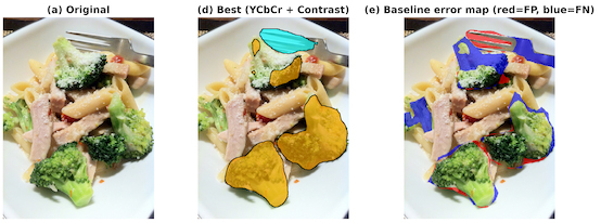
Augmentation-driven mask refinement on two representative scenes. Columns: (a) input, (b) ground truth, (c) sRGB/No-Aug baseline prediction, (d) YCbCr/Contrast prediction, and (e) baseline error map (red = FP, blue = FN). Top: metal (cyan) +fruits (orange). Bottom: glass (green) +paper (magenta). Improvements in (d) mirror the quantitative gains (Table III) and the latent-space separation (Fig. 11).

3.6

Where Augmentation Helps: Qualitative Evidence

Figure 12 provides two typical scenes to illustrate where the gains come from. Each row shows the input, ground truth, an sRGB/No-Aug baseline prediction, the best model (YCbCr/Contrast), and a baseline error map (red = FP, blue = FN). In the metal + fruits example (top), the baseline misses thin specular lobes and undersegments low-saturation fruit. The YCbCr/Contrast recovers these regions and removes spurious fragments, matching the Recall/IoU uplift in Table III and the cluster tightening in Fig. 11. In the glass + paper example (bottom), both classes are already relatively easy (high albedo, strong edges), yet augmentation still sharpens boundaries and heals small gaps—consistent with their higher-valued rows in Fig. 7.

3.7

Synthesis

Across analyses, three conclusions are consistent and mutually supporting:

(1)

Color space alone has limited impact. Global distributions (Fig. 6) and ANOVA (Table II) show small, nonsignificant main effects for color space on IoU/F1. Simple re-encoding does not change the photometric variability the network experiences.

(2)

Augmentation—especially Contrast—improves overlap metrics. Heatmaps (Fig. 8), EMMs (Table III), pairwise tests (Table IV), and IoU error bars (Fig. 10) are in agreement: Contrast significantly outperforms No-Aug and Saturation on IoU and F1, and improves Recall. Brightness can lift Precision but does not match Contrast on overlap metrics.

(3)

Dataset color statistics explain where gains appear. The broad chroma spread of fruits and the low-chroma, specular nature of metal in Fig. 3 predict the observed failure modes and improvements: YCbCr/Contrast compacts and separates these manifolds (Fig. 11), and recovers the corresponding pixels (Fig. 12). Per-material deltas (Table V) corroborate this mechanism.

Discussion

Augmentation dominates—when aligned with perceptual axes. Across our 3 × 4 design, augmentation is the main determinant of performance while the pixel encoding (color space) plays a secondary, modulatory role. The Type-III ANOVA (Table II) quantifies this (small, nonsignificant main effects), and the effect is visible in the model × material heatmap (Fig. 7) and the color space × augmentation summary (Fig. 8). The augmentation-level mixed-model EMMs (Fig. 10; Table III) reinforce the same ordering. Mechanistically, gains are largest when perturbations are expressed along opponent axes respected by both human vision and many vision pipelines: a single luminance dimension and two opponent-chromatic dimensions. The CIELAB and YCbCr factor images this way, letting us (i) modulate luminance statistics without corrupting hue and (ii) scale chroma magnitude at fixed hue. In contrast, edits in gamma-encoded sRGB entangle lightness and hue, which partly explains why sRGB adjustments yield smaller, less consistent benefits (Fig. 8). The BCE insensitivity to region overlap (Fig. 5) further motivates our reliance on the overlap-centric metrics in Section 2.3.

Color science of materials: why classes move (or do not) under specific augmentations. The per-material landscape (rows in Fig. 7) aligns with appearance physics and the training-set color statistics (Fig. 3). Metals and glass are specular-dominant: diagnostic energy is in luminance gradients, highlight–shadow transitions, and environment reflections. Luminance-centric perturbations (Brightness/Contrast) therefore teach invariance to illumination envelopes without distorting chroma, producing the largest IoU jumps for these classes (Table V; metal: +8.3 pp for Brightness, +5.9 pp for Contrast; glass: +7.9 pp/+5.1 pp). Qualitative overlays (Fig. 12, top) show YCbCr+Contrast recovering thin specular lobes missed by sRGB/No-Aug.

Fruits and paper are diffuse and chroma-dominant: separability is achieved by stable chromaticity with simpler shading. Saturation adjustment increases separation in a∗b∗ and CbCr, enlarging decision margins; accordingly, Saturation yields the largest gain for paper (+6.2 pp) and competitive gains for fruits (+3.9 pp), while Contrast still helps by sharpening albedo edges (Table V; Fig. 7). Figure 12 (bottom) shows how YCbCr+Contrast sharpens boundaries left jagged by the baseline.

Plastic straddles regimes: often near-neutral, weakly saturated, and glossy–diffuse. Here, YCbCr’s luma–chroma decorrelation provides a slight baseline advantage and small Contrast gains (Table V; Fig. 7), consistent with edges defined more by luminance than hue. Animal hair and feather are structurally challenging: fine strands and textures depress Recall (radar in Fig. 9); Contrast helps moderately but cannot fully overcome stride-16 thin-part losses (Table V). Ceramic behaves as glossy–diffuse: Contrast yields steady mid-sized gains; Saturation is mild (Table V).

Which pairings work best (and which to avoid). Aggregating across materials and color spaces, Contrast is the safest default (Figs. 8 and 10; Table III), improving IoU/F1 with minimal downside and significantly surpassing No-Aug/Saturation on IoU and F1 (Table IV). For specular classes (metal, glass), add Brightness along the luminance axis (YCbCr Y or CIELAB L∗) for the biggest jumps (Table V); Contrast is a close second. For chroma-dominant classes (paper, fruits), Saturation in CIELAB or YCbCr works well, with Contrast again a solid fallback. Two caveats: (i) Saturation on glass/metal can hurt (Table V) by creating false positives around colored reflections or transmitted tints; (ii) strong Brightness in CIELAB may compress L∗ contrasts and conflate light paper with shiny metal, a failure echoed in Fig. 7 and the error maps in Fig. 12(e). These behaviors are predicted by the dataset’s color statistics (Fig. 3): narrow chroma around the origin makes specular classes sensitive to chroma inflation; wide, saturated clusters make diffuse classes respond to chroma scaling.

Latent-space geometry: how augmentation reshapes separability. The t-SNE plots (Fig. 11) visualize how learned features reorganize under different training conditions. With sRGB/No-Aug, luminance and chroma remain entangled, producing tilted, overlapping clusters—mirroring the modest IoU in Fig. 8 and the overlapping distributions in Fig. 6. Moving to YCbCr partially disentangles axes; adding Contrast contracts the 95% ellipses and increases centroid separation—especially for materials whose cues align with luminance structure (metal/glass) or crisp albedo edges (paper). This progression suggests Contrast regularizes early filters around Michelson contrast while preserving chroma opponency, yielding features that generalize across illumination without sacrificing material chromaticity. The qualitative error reductions in Fig. 12 from baseline to YCbCr+Contrast are the spatial footprint of this latent compaction and separation, and they track the quantitative ordering in Figs. 8 and 10, and Table V.

Practical guidance. If a single policy must be chosen, train with Contrast in an opponent space (YCbCr or CIELAB). For deployments dominated by metal/glass, include Brightness adjustment on the luminance channel. For datasets rich in paper/fruits, add Saturation adjustment (preferably in CIELAB), but disable it for glass/metal regions to avoid chroma-induced false positives. Where neutral objects like plastic are prevalent, YCbCr baselines plus Contrast give consistent, if modest, gains.

Limitations and context. Object-centric COCO labels inject material noise in mixed objects, capping attainable IoU for heterogeneous classes (Section 2.1; Fig. 7). Unequal chromatic spreads across materials (Fig. 3) mean a fixed saturation step perturbs classes unequally, so per-material deltas (Table V) should be interpreted relative to each class’s native chroma variance. Early stopping keyed to BCE (Fig. 5) may slightly bias checkpoints away from overlap-optimal epochs; nevertheless, the ANOVA (Table II), EMMs (Fig. 10), and held-out metrics (Figs. 8 and 9) converge on the same conclusion: augmentation choice is the principal lever, and its benefits are maximized when applied in perceptually coherent color spaces. Finally, because our sRGB edits occur in the gamma-encoded domain (as per common libraries), “contrast” and “brightness” there are not identical to linear-light operations; this could slightly shift numeric effect sizes but does not affect our qualitative conclusions.

Conclusion

We set out to answer a focused question: Does the color space in which color augmentations are applied matter for material segmentation? By holding architecture and training constant and sweeping a 3 × 4 grid of color spaces and augmentation types (36 runs over three seeds) on a common 81-image test split, we decoupled augmentation from pixel encoding.

Three conclusions emerge.

(1)

Augmentation, not re-encoding, is the principal lever. Simply converting images to CIELAB or YCbCr (without color augmentation) leaves test-set medians for Precision/IoU/F1 essentially unchanged relative to sRGB (Fig. 6); the fixed-effects ANOVA finds only small, nonsignificant main effects (Table II). In contrast, the mixed-effects model reveals clear augmentation gains: EMMs averaged over color spaces place Contrast at the top for IoU/F1/Recall, while Brightness maximizes Precision (Table III); Holm-adjusted pairwise contrasts confirm that Contrast significantly outperforms No-Aug and Saturation on IoU and F1 (Table IV; Fig. 10). Aggregated heatmaps convey the same narrative (Fig. 8).

(2)

Color space modulates—rarely dominates—the effect of augmentation. Benefits are most consistent when perturbations align with perceptual axes (one luminance, two opponent-chroma channels). Expressing Contrast or Brightness on Y or L∗ sharpens boundaries without corrupting hue, yielding the row-wise increases seen across materials in Fig. 7. The CIELAB’s near-uniform a∗b∗ plane favors chroma edits on diffuse, colorful surfaces (e.g., paper), whereas YCbCr’s luma–chroma separation can aid near-neutral or mixed materials (e.g., plastic). The interaction remains modest in the inferential analysis (Table II), which explains the portability of a single augmentation policy across encodings (Fig. 8).

(3)

Material appearance predicts where gains occur, and the latent space reflects it. Per-material heatmaps (Fig. 7) and radar profiles (Fig. 9) show that luminance-centric edits (Brightness/Contrast) help specular classes (metal, glass) while chroma scaling helps chroma-dominant diffuse classes (paper, fruits); qualitative overlays visualize these corrections at the pixel level (Fig. 12). In the learned representation, t-SNE embeddings evolve from overlapping clusters under sRGB/No-Aug to compact, better-separated manifolds under YCbCr/Contrast (Fig. 11), indicating that measured gains arise from more discriminative internal features rather than output post-processing.

Practical guidance. Use Contrast as a safe default in an opponent color space (YCbCr or CIELAB). Add Brightness for specular-heavy data (metal/glass); include Saturation for chroma-dominant surfaces (paper/fruits), but avoid chroma inflation on nominally achromatic media to prevent false positives. These choices are consistent with global EMMs (Table III), significance tests (Table IV), and per-material trends (Fig. 7).

Resources and outlook. We release COCO–Materials (object-to-material mapping, splits, and color statistics; Section 2.1; Fig. 3) and an open-source analysis toolkit that reproduces our figures (e.g., Figs. 11 and 12). Although absolute ceilings are limited by object-centric labels and thin-part geometry (Section 3.1), the factorial design supports robust relative conclusions: augmentation strategy drives performance, and perceptually coherent color spaces make those augmentations work better. Future work should combine these data-centric gains with boundary-aware losses and higher-resolution decoders, and explore per-material, strength-adaptive augmentation schedules guided by each class’s chromatic statistics (Fig. 3).

References

1CaoG.JiangJ.BollegalaD.LiM.LuoS.“Multimodal zero-shot learning for tactile texture recognition”, Preprint, arXiv:2306.12705 (2023)

2ShiL.LiB.HašanM.SunkavalliK.BoubekeurT.MěchR.MatusikW.2020MATch: differentiable material graphs for procedural material captureACM Trans. Graph.391151–1510.1145/3414685.3417815Article 271

3FlemingR. W.2017Material perceptionAnnu. Rev. Vis. Sci.3365388365–8810.1146/annurev-vision-102016-061429

4UpchurchP.NiuR.2022A dense material segmentation dataset for indoor and outdoor scene parsingComputer Vision — ECCV 2022Lecture Notes in Computer Science13668450466450–66Springer Nature SwitzerlandCham, Switzerland

5FinlaysonG. D.2018Colour and illumination in computer visionInterface Focus82018000810.1098/rsfs.2018.0008

6ShortenC.KhoshgoftaarT. M.2019A survey on image data augmentation for deep learningJ. Big Data66010.1186/s40537-019-0197-0

7Bello-CerezoR.BianconiF.FernándezA.GonzálezE.Di MariaF.2016Experimental comparison of color spaces for material classificationJ. Electron. Imaging2506140610.1117/1.JEI.25.6.061406

8CubukE. D.ZophB.ManeD.VasudevanV.LeQ. V.2019AutoAugment: learning augmentation policies from dataProc. IEEE/CVF Conf. Computer Vision and Pattern Recognition (CVPR)113123113–23IEEEPiscataway, NJ10.1109/CVPR.2019.00020

9DeK.PedersenM.2021Impact of colour on robustness of deep neural networksProc. IEEE/CVF Int’l. Conf. on Computer Vision Workshops (ICCVW)213021–30IEEEPiscataway, NJ10.1109/ICCVW54120.2021.00009

10AbebeM. A.ShahbaznejadS.RabbanifarA.FedorovskayaE.2025Unveiling the role of color in skin segmentation: analysis of augmentation techniques and color spacesJ. Imaging Sci. Technol.6905050410.2352/J.ImagingSci.Technol.2025.69.5.050504

11RitchieJ. B.PaulunV. C.StorrsK. R.FlemingR. W.2021Material perception for philosophersPhil. Compass16e1277710.1111/phc3.12777

12StorrsK. R.AndersonB. L.FlemingR. W.2021Unsupervised learning predicts human perception and misperception of glossNat. Hum. Behav.5140214171402–1710.1038/s41562-021-01097-6

13Bello-CerezoR.BianconiF.FernándezA.GonzálezE.Di MariaF.2016Experimental comparison of color spaces for material classificationJ. Electron. Imaging2506140610.1117/1.JEI.25.6.061406

14Bello-CerezoR.BianconiF.FernándezA.GonzálezE.Di MariaF.2016Experimental comparison of color spaces for material classificationJ. Electron. Imaging2506140610.1117/1.JEI.25.6.061406

15GeirhosR.RubischP.MichaelisC.BethgeM.WichmannF. A.BrendelW.2019ImageNet-trained CNNs are biased towards texture; increasing shape bias improves accuracy and robustnessInt. J. Comput. Vis.128261826382618–38

16DeK.PedersenM.2022Exploring effects of colour and image quality in semantic segmentation by deep learning methodsProc. Color and Imaging Conf. (CIC)111116111–6IS&TSpringfield, VA10.2352/J.ImagingSci.Technol.2022.66.5.050401

17LongJ.ShelhamerE.DarrellT.“Fully convolutional networks for semantic segmentation,” Proc. IEEE Conf. Computer Vision and Pattern Recognition (CVPR) (IEEE, Piscataway, NJ, 2015), pp. 3431–3440

18LinT.-Y.MaireM.BelongieS.HaysJ.PeronaP.RamananD.ZitnickC. L.DollárP.2014Microsoft COCO: common objects in contextComputer Vision — ECCV 2014Lecture Notes in Computer Science8693740755740–55SpringerCham10.1007/978-3-319-10602-1_48

19BuslaevA.IglovikovV. I.KhvedchenyaE.ParinovA.DruzhininM.KalininA. A.2020Albumentations: fast and flexible image augmentationsInformation1112510.3390/info11020125

20IEC 61966-2-1: Multimedia Systems and Equipment—Colour Measurement and Management—Part 2–1: Colour Management—Default RGB Colour Space—sRGB (1999)

21PoyntonC.Digital Video and HD: Algorithms and Interfaces20122nd ed.Morgan Kaufmann/ElsevierWaltham, MA, USA

22ITU-T Recommendation T.871. Information Technology—Digital Compression and Coding of Continuous-tone Still Images: JPEG File Interchange Format (JFIF) (2011)

23ITU-R Recommendation BT.601. Studio Encoding Parameters of Digital Television for Standard 4:3 and Wide-Screen 16:9 Aspect Ratios (2011)

24Commission Internationale de l’Éclairage. Colorimetry. 3rd ed., CIE 015:2004 (Commission Internationale de l’Éclairage, Vienna, Austria, 2004)

25FairchildM. D.Color Appearance Models20133rd ed.WileyChichester, UK

26MontagE. D.BernsR. S.2000Lightness dependencies and the effect of texture on suprathreshold lightness tolerancesColor Res. Appl.25241249241–910.1002/1520-6378(200008)25:4<241::AID-COL4>3.0.CO;2-E

27TielemanT.HintonG.Lecture 6.5—RMSProp: Divide the Gradient by a Running Average of Its Recent Magnitude2012

28PrecheltL.1998Early stopping—but when?Neural Networks: Tricks of the TradeLecture Notes in Computer Science1524556955–69SpringerBerlin/Heidelberg, Germany

29EveringhamM.Van GoolL.WilliamsC. K. I.WinnJ.ZissermanA.2010The PASCAL visual object classes (VOC) challengeInt. J. Comput. Vis.88303338303–3810.1007/s11263-009-0275-4

30DiceL. R.1945Measures of the amount of ecologic association between speciesEcology26297302297–30210.2307/1932409

31RahmanM. A.WangY.2016Optimizing intersection-over-union in deep neural networks for image segmentationAdvances in Visual ComputingLecture Notes in Computer Science10072234244234–44Springer International PublishingCham, Switzerland10.1007/978-3-319-50835-1_22

32WangZ.NingX.BlaschkoM. B.2023Jaccard metric losses: optimizing the Jaccard index with soft labelsAdvances in Neural Information Processing Systems (NeurIPS)Curran Associates, Inc.Red Hook, NY, USA

33SalehiS. S. M.ErdogmusD.GholipourA.2017Tversky loss function for image segmentation using 3D fully convolutional deep networksMachine Learning in Medical ImagingLecture Notes in Computer Science10541379387379–87Springer International PublishingCham, Switzerland

articleview.keywords